You might not have noticed from the extremely professional façade I portray on here, but in the last couple of years I’ve picked up the extremely fun and rewarding hobby of handball. It has become a really large part of my life, so much so that I interrupted my PhD from July through December this year because of it. Let me show you why.
Club champs
In July I competed for the UQ Handball Club at the Australia and Oceania Club Championships for the second time. And unlike last year, where I sat on the bench and eagerly absorbed as much as I could from the side-lines, another year of training (and the fortune of being the only left-hander on the team) earned me the responsibility of serious playtime. Five tough games later, we managed to pull off something the club had been working towards for the better part of a decade – toppling Sydney Uni, the reigning champions since 2014, and winning the final against St. Kilda.
This also earned us the right to compete at the 2023 IHF Super Globe, the annual handball club world championships held in November. Celebration soon turned to anticipation as we realised the hard work and sacrifice we would have to put in to mix it with some of the best professional clubs in the world.
Prep
With just over three months to prepare, we had to get started straight away. Four on-court trainings, three gym sessions and three running sessions each week is a lot to ask of people who otherwise still have full-time jobs and families. To me, I could see no way to balance this with tutoring and PhD work. I had committed to a lot of tutoring and semester had already started, so the PhD had to go. I made the arrangements to pause the PhD, and committed to this potentially once-in-a-lifetime opportunity. I’m very grateful to my supervisors and course co-ordinators for being flexible, supporting and understanding.
The preparation was tough, but by the end of the program I felt stronger, fitter and a lot better at handball. Of course, I learned a lot about myself and what motivates me to work hard, so it was a worthwhile experience for that reason alone.
The competition
It was always going to be tough playing against some of the best players in the world, especially when we hadn’t played on a stage like this before. There were a lot of firsts: first time playing in front of thousands of spectators, all supporting the other team; first time getting a police escort; first time playing against professionals; first time losing by 40+ goals. But you learn a lot about how you can improve in these situations, so we’re excited to work hard to do it all again next year. We set ourselves a benchmark, and showed that an Australian-based team can perform on the world stage.
What I learned
Individually, I know I have a lot to work on over the next twelve months to help the team get back to this position next year, and then give a better showing of myself if we get there. I learned to be resilient in times of adversity, and I learned what matters to me and how to better manage my time next year so I can manage my PhD as well as handball. (Farewell tutoring!) Finally, I learned to embrace opportunities when they arise, and enjoy every moment.
What follows is the academic residue of a spirited discussion between a fellow PhD student and myself, concerning the use of measure theory in probability. The central question is “Why bother?” Here is my attempt at an answer to this question, through a small demonstration of measure theory’s ability to generalise. This is not an attempt to teach any measure theory, but I will point to a few resources at the end that I found helpful for reacquainting myself during our discussion if you would like to do the same.
The traditional result
First, we must establish in traditional terms the result we will later emulate measure-theoretically. I will only talk about non-negative random variables; the result generalises by splitting into positive and negative parts, but the notation is drastically simplified.
Theorem 1: If is a non-negative random variable with density and probability function , then .
Proof:
There are two conceptually important points here. The less theoretically troublesome one is the switching of integrals, which Fubini lets us do, but I’ve always found a little cheeky. More foundationally important is that we assume the existence of a density here, but it is absent from the result of the theorem. It is an achievable exercise to prove the equivalent result for discrete distributions, and I concede that most continuous distributions I have encountered in the wild have a density, but this does have practical importance. The usefulness of the theorem is in being able to compute an expectation when we don’t have or don’t want to find a density, so it’s essentially useless if having a density is a pre-condition to its application. Can we get around this somehow?
In steps measure theory
I will spare the majority of the details of satisfactorily defining a random variable measure-theoretically, but some objects need to be defined.
The premise of measure-theoretic probability is that we start with a measure space . In probability terms, this gives us a sample space, a set of events and a probability measure, as long as . We will brush over what is really saying, but suffice to say it imposes Kolmogorov’s unit measure axiom. The other axioms of probability are packaged up in what a measure space is. This gives us a notion of what probability means on . We can then define a real-valued random variable as a measurable function from to the reals, that is, a function such that the pre-image of any open interval is an element of .
For our purposes, we can define any real-valued random variable as follows, by first defining the distribution. Take to be our measure space, where is the set of Lebesgue-measurable subsets of , and is the Lebesgue measure. Then the uniform distribution can be defined as the identity map . You can check for yourself that any property you like about the uniform distribution carries over perfectly. In particular, we can check that .
Now, anyone familiar with the inverse-transform will know that defining any other real-valued random variable is a piece of cake. Every real-valued random variable has a distribution function , so we define . might not be easy to compute, but it definitely exists.
We are still missing one key element, expected value. We define it as . I will leave undefined what it means to actually compute an integral this way, but it can be done. Importantly, it is still achieving the same goal of finding area under a curve. We are now ready to prove:
Theorem 2: If is a non-negative random variable with probability function , then .
Proof:
If you’ll allow me a couple of pictures, I argue that it is true by definition. We see that the area integrated by and the area integrated by are in fact the same areas.
.
.
Q.E.D.
Some healthy skepticism
Now, we should be skeptical of any proof which follows so readily from the definitions. The traditional discrete distribution is marvelously intuitive. Further, we can squint at the traditional continuous expected value definition and notice the pattern. By comparison, the measure-theoretic definition is quite opaque. So far it seems like we just made up a definition so that this proof was easy. What’s the value in that? Here’s how I see it.
I liken it to the intermediate value theorem (IVT). The point of proving the IVT is not to dispel any doubt that if an arrow pierces my heart it must also have pierced my ribcage. The point of the IVT is in showing that the definition of mathematical continuity we have written down captures the same notion of physical and temporal continuity we sense in the real world.
What we have really learned from theorem 2 then, is that we can define expected value in terms of the probability function directly. We essentially drop the density assumption by fiat. The value is in discovering this more powerful definition which unites previously disparate discrete and continuous cases, as well as distributions which are a mix of both.
A concrete mixed distribution example
My favourite mixed distribution is the zero-inflated exponential, with probability function when , and otherwise.
Traditionally, to evaluate an expected value we would have to be rather careful or apply some clever insight. Now with measure theory, we can ham-fistedly shove straight in to and call it a day.
We can also start sparring with more exotic random variables on non-numeric spaces with confidence. I’m currently working through Diaconis’ Group Representations in Probability and Statistics, so hopefully I can speak on these “applications” in more detail in the future. But for now, I’ll leave it as an enticing mountaintop rather than trying to spoil the ending.
Intuition
It is no secret that I don’t like the IVT, or theorem-motivated definitions more broadly, so I am uncomfortable leaning on it in an argument. What I will provide here is my own post-hoc intuition for the measure-theoretic expected value. Rather fortuitously it leans on the IVT, so I’ll point out pedantically that I’m actually using it as the Intermediate Value Property (IVP) in and of itself. Observe below that the area on the left is the area defining a measure-theoretic expected value as we have seen above.
The area defining a measure-theoretic expected value, and the rectangular region of equal area guaranteed by the IVP.
Note that this area is the same as the area of the rectangular region. As it has unit width, its height is also its area. This height is not coincidentally the mean value of guaranteed by the IVP, so we see that the measure-theoretic definition gives us a measure of central tendency. That this is the same measure of central tendency as the traditional definition can be shown in many ways, but we have seen it today as a porism of theorem 2.
What have we learned?
In short, that generalisation is cool, and measure theory is not as scary as I thought after failing it in third-year. It gives us steady footing to go and explore exotic spaces, and it provides some nice perspectives on old favourites. Is it of practical use to the working statistician? Debateable. Our main theorem can certainly be used without actually doing any measure. Perhaps it provides nice perspectives on transformations if one does need to compute certain integrals which aren’t recognisable. What do you think? Have I convinced you measure-theoretic probability isn’t useless? Do you know any interesting applications I didn’t mention? As always, I’d love to hear your thoughts.
Resources
I am always hesitant to endorse texts based solely on how helpful they were to me. We should remember that one always understands something better the second time. That being said, the following two probability-oriented texts were useful to me. Matthew N. Bernstein has a trio of nice blog posts entitled Demystifying measure-theoretic probability theory, which are a nice, slow introduction to some of the basics. I also found Sebastien Roch’s Lecture Notes on Measure-theoretic Probability Theory useful as a much denser, more comprehensive reference. As for strictly measure-theoretic principles, I found plenty enough information by simply clicking the first Wikipedia article to pop up when I searched the relevant terms.
We want to roll dice at a time, and add up the total over repeated rolls, and continue to do so until we reach a threshold . When we reach or exceed , we note , the sum of the dice we just rolled. What is the distribution of ? We will call the range to the striking range, as a roll in this range might get us to . Inside this range we need to pay extra attention to the value of our dice roll, as depending on its value we might have to roll again, or we might have to stop.
Let be the cumulative sum of dice rolled times. Let be the cumulative sum of dice rolled an unknown number of times. We want to find a mixing point after which is uniform in terms of . Why? If we find such an , then as long as our threshold is at least a few maximum dice rolls away from , it doesn’t really matter how far away it is, we can always assume our cumulative total approaches the striking range from somewhere uniformly in an appropriately wide interval just outside the striking range. This significantly reduces the complexity of an analytic solution or a computer simulation. If the threshold is not significantly past the mixing point, then we have to be careful as our cumulative total is more likely to be at particular points, and the calculations become more complex, as our cumulative total will come in chunks of about at a time.
Does M exist?
It might be that doesn’t really exist, and there is always some very subtle nonuniformity to . This isn’t necessarily the case, but showing that would be another problem entirely, and we’re probably quite fine with technically a function of some tolerance level. Let’s quickly develop a mental picture with some histograms. This will hopefully convince us that exists (or we get close enough to uniform that it looks like exists), and how we might capture its meaning.
Pictures
For a particular set of and , just follows some discrete distribution with a nice bell-curvy shape. Of real interest is sampling from , as we don’t know how many rolls it took to reach our threshold. The immediate problem is this requires sampling a first, and we don’t want to have any assumption on ‘s value. So instead I will just uniformly sample values between 0 and 200 and hope that our brains can imagine the extension to unbounded . Play around with my code in the Colab notebook here. Actually, let’s always sample but keep track of the partial sum at each intermediate step. I know this technically violates independence assumptions, but whatever. I’m also going to work with for these pictures, as the results are suitably interesting.
Here we can see a histogram for 10 000 samples of . As expected it forms a lovely bell-curve shape.
Here we see a histogram for 10 000 samples of for all . We can see the nice uniform property we’re looking for emerge definitively once exceeds about 3 000, but it’s hard to tell at this scale. Let’s zoom in on the more interesting part of the graph.
Here we only look at samples of for . We can see more clearly now the spikes which indicate we are not at the mixing point yet, which we can make out more clearly here is at about . Zooming in further:
We can identify the spikes more clearly here. Given we roll 20 dice at a time, we should not be surprised to see the initial values occur in spikes about 70 units apart, which is roughly what we see.
They do get a bit wider as we move to the right, as the tails of slightly fatter and further right spikes gently nudge up their neighbours. So, whatever more technical answer we derive below should line up roughly with these observations, namely that by the time is about 2000, or about 29 dice rolls, it should be well mixed.
Defining M
For a more technical definition, you can be as picky as you like as to how you define suitably uniform, probably with some sort of floating around, but I want a rough and ready answer, and I don’t personally enjoy having ‘s littered throughout my work, so my working definition is as follows:
If, for all , it is no longer obvious to infer from how many rolls it took to reach , then is a mixing point.
Of course this is entirely heuristic, it is not longer obvious (in some sense) as long as there is more than one value for which is nonzero. This happens very quickly and does not capture what we see in the simulations. In the other direction, for any , there will always be some much more sensible guesses for than others, probably an integer close to . So we need to start by deciding on our criteria for obvious. I’ve come up with a couple of different definitions, and I’ll discuss them both below.
Finding M the easier way
It can be checked that , and that . From now on, if I need to, I will approximate with , a normal random variable with the same mean and variance. Then I can say we have reached the mixing point if there is significant overlap between and for some . Again there are lots of choices for what is meant by significant overlap and choice of . Inspired by mathsfeed.blog/is-human-height-bimodal I think a reasonable choice is to compare , and consider the overlap significant if the there is only one mode, not two. Using the fact that a normal pdf is concave down within 1 standard deviation of its mean, we would like that one standard deviation above the mean for :
is equal to one standard deviation below the mean for :
One can do some rather boring algebra to arrive at . You can solve this properly I guess, but I am a deeply lazy person, so I’m going to approximate the right-hand side as . If this upsets you, then I am deeply sorry, but I will not change. ( is big enough and we’re rounding to a whole number at the end of the day so its fine, but I’ve already spent more time justifying this than I wanted to.) This allows us to arrive at . This roughly agrees with the scale we wanted for . If you try and count out the first 21 spikes in the above plots, they become very hard to make out by the end. So I’m actually fairly happy with this answer, subject to some proper checking with more choices for and maybe just topping off with another 20% just for good measure. More important I think is convincing yourself that if I had chosen some other number of standard deviations or some larger , then as a function of should still be linear! So instead of rederiving all of these calculations, just remember that if you’re happy , is well-mixed, then , should be well-mixed too. Note that this condition truly isn’t enough to guarantee uniformity as it makes no attempt to consider the contribution of any other than and , but it should ensure any spikiness is rather muted. If you’re happy with this condition, good, so am I, but I may as well mention the other method I thought of for measuring mixing.
Finding M the bayesian way
The definition of suitably uniform above is very heavily based in conditional probability, and I am a dyed-in-the-wool bayesian, so I’m going to attack with all the bayesian magic spells I can muster. If you’re a committed frequentist, maybe it’s time to look away.
We want to derive
.
Can we derive ? Well by the definition of conditional probability,
.
I know is approximately normal, so
,
and we have no prior information about what should be, so we can treat with a constant uninformative prior. Finally, is not a function of , its just a scaling factor, so
.
Now admittedly it’s been a while since I was properly in the stats game, so my tools might be a bit rusty, but this doesn’t look like a pmf I’m familiar with. It looks like it’s in the exponential family, so maybe somebody with more experience in the dark arts can take it from here. I guess you could always figure out some sort of acceptance-rejection sampler if needed. Okay but what’s the point? Well now we have our posterior for , we can be more precise about it being suitably non-obvious what to infer for . The first criteria that come to mind for me is either specifying the variance should be suitably large (which can be approximated up to proportionality with the pdf, though that proportionality depends on generally), or that the mode of the distribution is suitably unlikely (also easy up to proportionality, but knowing the actual probability itself feels more integral to the interpretation). Of course in both cases we can approximation the proportionality constant by computing an appropriate partial sum. I’ve knocked up a quick demo on Desmos of what this would look like in practice.
Concluding remarks
Note of course that the normal approximation itself only works if the number of dice in each roll is suitably large to apply CLT. It also then feels like no coincidence that ‘about 30 rolls’ is the conclusion, as it sounds an awful lot like my usual usual retort when asked if a sample mean is big enough to make a normal approximation. Overall I’m okay with making approximations which assume a large for the same reason we are more interested in deriving results for large , namely for small and/or , we can probably simulate the answer with high precision using a computer, or even by hand for very small values. But these asymptotic results help us to be confident in when we can truncate the simulation for speed, or when we can stop doing simulations and rely only on the asymptotic results.
My hope is that this post distills the interesting unanswered questions from my honours thesis. The final question relies on various results and definitions which I will try to introduce in the most interesting way possible, occasionally avoiding formalism if it conflicts with reader enjoyment and intuition. I will try and title broad sections so those already familiar can skip if they want to rush ahead. I will assume you are already familiar or able to look up basic graph theory notations and definitions. If ever you crave more of the gruesome details, they are of course to be found in the thesis.
Hamilton decomposition of a finite graph
Here we see , the complete graph on 5 vertices. The edges have been coloured so that the edges of one colour form a spanning, 2-regular subgraph. Each colour is called a Hamilton cycle, and the colouring of the graph is called a Hamilton decomposition. A Hamilton cycle provides a path which visits every vertex exactly once and returns to the starting vertex.
The natural question for a given graph is whether or not it has a Hamilton decomposition. The obvious criteria are that the graph must be connected, and even-regular. The less obvious necessary condition is a refinement of the connected condition; more precisely, a -regular graph must be -edge connected, i.e. there is no set of edges which, upon deletion, make the graph disconnected.
Exercise: Prove this necessary condition.
A graph which fits the necessary criteria will be called admissible. If every admissible graph had a Hamilton decomposition, then we would be done, but we know of examples where this is not the case, even if we assume a high level of structure in the graph. In general it is still hard to tell if an admissible graph has a Hamilton decomposition, but there are some lovely families of admissible graphs for which we do know a Hamilton decomposition.
One family of graphs for which we know a lot is the Cartesian product of two graphs and . (wiki) At each vertex of , insert a copy of , and connect equivalent vertices of when they in adjacent vertices of .
Exercises: Check that is isomorphic to . Check that if is -regular and is -regular, then is -regular.
Exercise: (for those who are familiar with graph automorphisms) Verify that .
Of relevance for us are the following results:
Kotzig 1973 [1]: The Cartesian product of two cycles has a Hamilton decomposition.
Foregger 1978 [1]: The Cartesian product of three cycles has a Hamilton decomposition.
Aubert and Schneider 1982 []: If is a 4-regular graph with a Hamilton decomposition, then has a Hamilton decomposition.
There are stronger results, culminating with Stong (1991) [3], but these results are enough for us to forge ahead towards our final problem.
Hamilton decomposition of an infinite graph
We borrow the interpretation of a Hamilton cycle in a finite graph as a spanning 2-regular subgraph. This no longer forms a cycle then, as such a cycle would only visit a finite number of vertices, it instead forms a path. We call such a path in an infinite graph a Hamilton double-ray. Then a Hamilton decomposition of an infinite graph is a colouring of the edges so that every colour is a Hamilton double-ray. We will denote by the graph which every Hamilton double-ray is isomorphic to.
The Hamilton decomposition of the -distance graph, which has the integers as vertices, and an edge between two vertices iff .
The Hamilton decomposition of the 2-dimensional lattice.
Observe in the above two examples some lovely properties. In the distance graph, we have the same chunk of colouring repeated every 6 units, a clever exploitation of the sliding symmetry of the integers. Similarly in the lattice, each colour is self-symmetric under a 180º-rotation, and the two colours are each a 90º-rotation of the other, cleverly exploiting the rotational symmetry of the lattice. I find this to be such a simple and lovely picture, I can’t believe this would be a 21st century observation. Like the six-petal rosette, it should have been noticed countless times throughout history, perhaps a Girih in a Syrian shrine, or painted onto an ancient roman pot. Art historians please get in touch. Otherwise, we should pin down a key difference in the structure of these two infinite graphs.
The six-petal rosette is the starting point for another infinite graph with its own lovely Hamilton decomposition.
Ends of infinite graphs
Informally, we can think of an end of a graph as a distinct direction into which our graph can extend infinitely. Slightly less informally, we say two ends are different if there is some finite vertex-deletion which makes the two ends disconnected. Then we can say that the number of ends of a graph is the maximum number of infinite connected components under some finite vertex-deletion. Then any finite graph has 0 ends. What are other possible values for the number of ends of a graph? The distance graph has 2, deleting a reasonably large chuck of vertices in the middle will produce two infinite connected components, one on the left (a negative end) and one on the right (a positive end). It might seem at first that the lattice has many, corresponding to different angles of escape, but in fact it only has 1. Any finite deletion of vertices might leave some finite components in the middle, but will never leave two infinite connected components. A graph can certainly have more than 2: taking the -star graph and extending each leaf indefinitely produces a -ended infinite graph, for example. But if a graph does have more than two, we could never hope to visit every vertex in that graph with a single Hamilton double-ray, some end would always be left out. This explains the differing patterns between our two exemplars above. As the distance graph has two ends, and so does a Hamilton double-ray, we can extend each end of the double-ray into each end of the graph quite comfortably. Whereas for the one-ended lattice, we have to carefully wrap our two ends up in a spiralling fashion to, in a sense, make a thicker one-ended spiral.
Extra necessary conditions
Unfortunately, there is another obstacle which arises when we begin to consider such infinite graphs. As well as requiring no more than 2 ends, if the graph is one-ended, there may be a parity issue as to why no decomposition can exist. Consider the following two-ended graph :
.
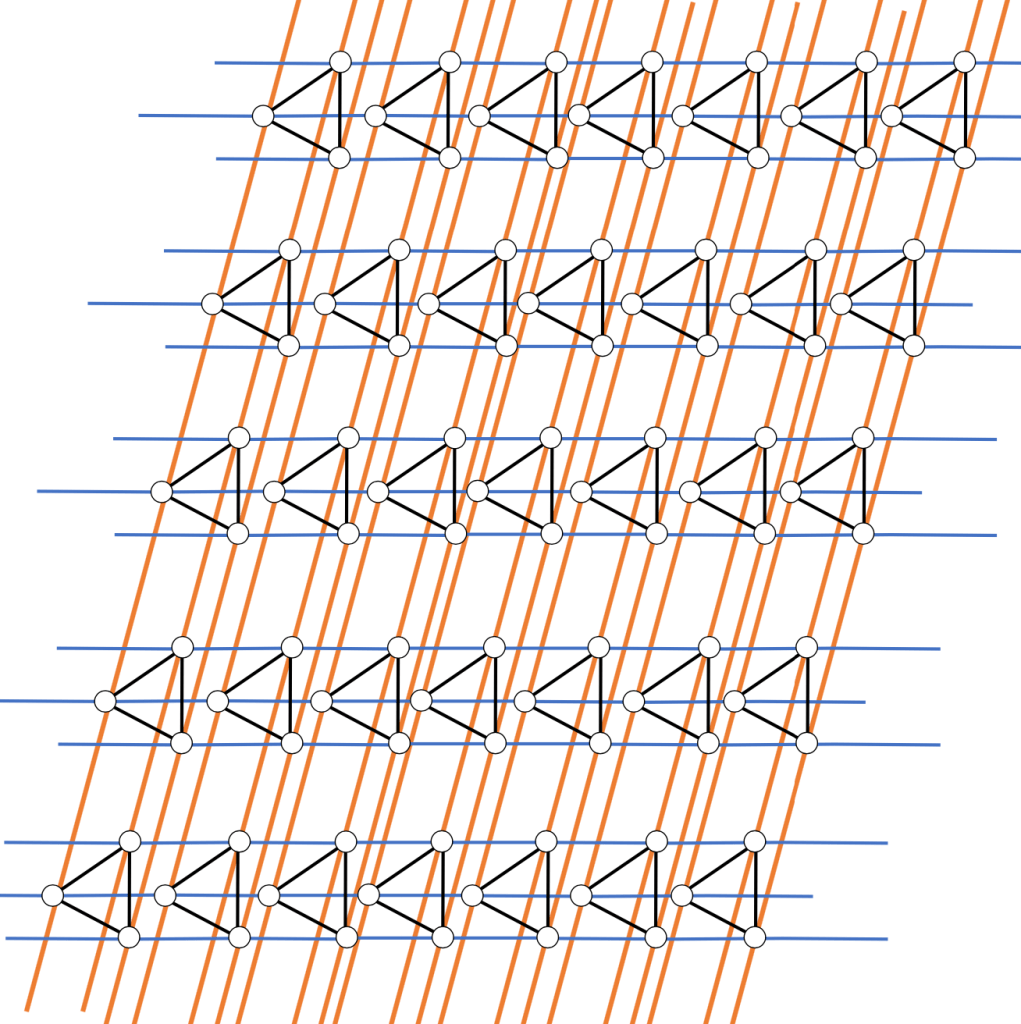
Note the three dotted edges. Each Hamilton double-ray must pass through this edge-set an odd number of times, as otherwise it would have both its ends on the same side of the graph, which in turn would mean it only visits a finite number of vertices on the other side. As this graph is 4-regular, it would be decomposed into two Hamilton double-rays. Two odds add to an even, but there are 3 edges, so clearly this is not possible. This argument can be generalised and refined in the case where our two-ended graph is of the form , namely, a Hamilton decomposition is only possible if is even. What a relief it is then, that it is always possible if is even. The below image suggests the pattern we can apply in such a case.
The Hamilton decomposition of .
The big questions
Erde, Lehner and Pitz 2020 [4]: If and are infinite, finite-degree graphs, each with a Hamilton decomposition into double-rays, then has a Hamilton decomposition into double-rays.
.
In general, it would be nice if has a Hamilton decomposition, this would be a nice generalisation of Foregger’s and Aubert and Schneider’s results for finite graphs, either viewing as an infinite cycle in which case Foregger’s result would apply, or by viewing as the lattice which already has a Hamilton decomposition, in which case Aubert and Schneider’s result would apply. If is even, then we already know that has a Hamilton decomposition as above, so we can use Erde, Lehner and Pitz’s result to then say that has a Hamilton decomposition. If is odd, then doesn’t have a Hamilton decomposition, so we can’t approach it this way. We already know it’s possible for one odd case, namely , in which case we simply have the lattice. Understanding any symmetry and pattern in the even case would be incredibly insightful for determining the odd case, but the construction becomes a bit too complex, and the pictures a bit too messy, that it would take a very careful hand to draw out the decomposition in a way we could wrap our heads around it. If you can manage to draw out the decomposition for , this would already be a more concrete example than anything I have managed to draw, and probably provide quite a valuable mental image of how to translate this to odd . Alternatively, it seems that the simplest odd case has all the right components for its own lovely symmetric solution, given that a decomposition would have 3 colours and the graph has an order 3 symmetry. Such a solution would provide its own insight into the other odd cases. So there is no reason a clever human brain couldn’t figure out a nice solution directly, perhaps inspired by the lattice decomposition. Alas, so far it seems that clever human brain might not be mine, but it might be yours!
Bibliography
[1] Marsha F. Foregger. Hamiltonian decompositions of products of cycles. Discrete Mathematics, 24:251–260, 1978. [2] Jacques Aubert and Bernadette Schneider. Decomposition de la somme cartesienne d’un cycle et de l’union de deux cycles hamiltoniens en cycles hamiltoniens. Discrete Mathematics, 38:7–16, 1982. [3] Richard Stong. Hamilton decompositions of Cartesian products of graphs. Discrete Mathematics, 90:169–190, 1991. [4] Joshua Erde, Florian Lehner, and Max Pitz. Hamilton decompositions of one-ended Cayley graphs. Journal of Combinatorial Theory, B(140):171–191, 2020.


 is a non-negative random variable with density
  and probability function
  , then
  .
. 
 . In probability terms, this gives us a sample space
  , a set of events
  and a probability measure
  , as long as
  . We will brush over what
  such that the pre-image
  of any open interval
  is an element of
  distribution. Take
 ![\left(\left[0,1\right], \lambda\left(\left[0,1\right]\right), \mu \right)](https://s0.wp.com/latex.php?latex=%5Cleft%28%5Cleft%5B0%2C1%5Cright%5D%2C+%5Clambda%5Cleft%28%5Cleft%5B0%2C1%5Cright%5D%5Cright%29%2C+%5Cmu+%5Cright%29&bg=ffffff&fg=7f8c8d&s=0&c=20201002) to be our measure space, where
to be our measure space, where ![\lambda\left(\left[0,1]\right]\right)](https://s0.wp.com/latex.php?latex=%5Clambda%5Cleft%28%5Cleft%5B0%2C1%5D%5Cright%5D%5Cright%29&bg=ffffff&fg=7f8c8d&s=0&c=20201002) is the
is the ![\left[0,1\right]](https://s0.wp.com/latex.php?latex=%5Cleft%5B0%2C1%5Cright%5D&bg=ffffff&fg=7f8c8d&s=0&c=20201002) , and
, and  is the
  can be defined as the identity map
 ![U: \left[0,1\right] \to \left[0,1\right] ; U(\omega) = \omega](https://s0.wp.com/latex.php?latex=U%3A+%5Cleft%5B0%2C1%5Cright%5D+%5Cto+%5Cleft%5B0%2C1%5Cright%5D+%3B+U%28%5Comega%29+%3D+%5Comega&bg=ffffff&fg=7f8c8d&s=0&c=20201002) . You can check for yourself that any property you like about the uniform distribution carries over perfectly. In particular, we can check that
. You can check for yourself that any property you like about the uniform distribution carries over perfectly. In particular, we can check that  .
.  , so we define
 ![X : \left[0,1\right] \to \mathbb{R}; X(\omega) =F_X^{-1} \circ U(\omega) = F_X^{-1}(\omega)](https://s0.wp.com/latex.php?latex=X+%3A+%5Cleft%5B0%2C1%5Cright%5D+%5Cto+%5Cmathbb%7BR%7D%3B+X%28%5Comega%29+%3DF_X%5E%7B-1%7D+%5Ccirc+U%28%5Comega%29+%3D+F_X%5E%7B-1%7D%28%5Comega%29&bg=ffffff&fg=7f8c8d&s=0&c=20201002) .
.  might not be easy to compute, but it definitely exists.
  . I will leave undefined what it means to actually compute an integral this way, but it can be done. Importantly, it is still achieving the same goal of finding area under a curve. We are now ready to prove:
  and the area integrated by
 ![\int_{\left[0,1\right]} F^{-1} \mathop{d\mu}](https://s0.wp.com/latex.php?latex=%5Cint_%7B%5Cleft%5B0%2C1%5Cright%5D%7D+F%5E%7B-1%7D+%5Cmathop%7Bd%5Cmu%7D&bg=ffffff&fg=7f8c8d&s=0&c=20201002) are in fact the same areas.
are in fact the same areas. 

 when
when  , and
, and  otherwise.
  and call it a day.

 dice at a time, and add up the total over repeated rolls, and continue to do so until we reach a threshold
  . When we reach or exceed
  to
to  the striking range, as a roll in this range might get us to
  be the cumulative sum of
  times. Let
  be the cumulative sum of
  after which
  is uniform in terms of
  . Why? If we find such an
  at a time.
  . This isn’t necessarily the case, but showing that would be another problem entirely, and we’re probably quite fine with
  but keep track of the partial sum at each intermediate step. I know this technically violates independence assumptions, but whatever. I’m also going to work with
  for these pictures, as the results are suitably interesting.
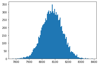
 . As expected it forms a lovely bell-curve shape.
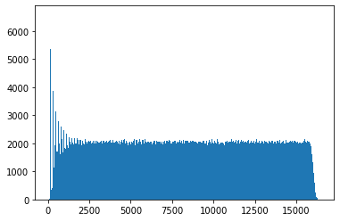
 for all
  . We can see the nice uniform property we’re looking for emerge definitively once
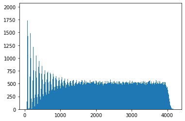
 . We can see more clearly now the spikes which indicate we are not at the mixing point yet, which we can make out more clearly here is at about
  . Zooming in further:
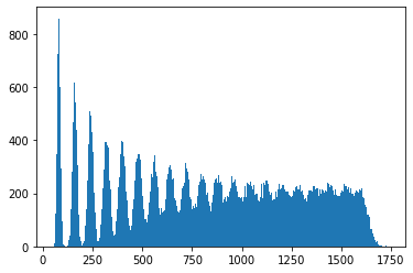
 floating around, but I want a rough and ready answer, and I don’t personally enjoy having
  , it is no longer obvious to infer from
  is nonzero. This happens very quickly and does not capture what we see in the simulations. In the other direction, for any
  . So we need to start by deciding on our criteria for obvious. I’ve come up with a couple of different definitions, and I’ll discuss them both below.
  , and that
  . From now on, if I need to, I will approximate
  , a normal random variable with the same mean and variance. Then I can say we have reached the mixing point if there is significant overlap between
  for some
  . Again there are lots of choices for what is meant by significant overlap and choice of
  . Inspired by
  , and consider the overlap significant if the there is only one mode, not two. Using the fact that a normal pdf is concave down within 1 standard deviation of its mean, we would like that one standard deviation above the mean for
 :
: 
 . You can solve this properly I guess, but I am a deeply lazy person, so I’m going to approximate the right-hand side as
  . If this upsets you, then I am deeply sorry, but I will not change. (
 . This roughly agrees with the scale we wanted for
  ,
,  is well-mixed, then
  ,
,  should be well-mixed too. Note that this condition truly isn’t enough to guarantee uniformity as it makes no attempt to consider the contribution of any
  other than
  and
and  , but it should ensure any spikiness is rather muted. If you’re happy with this condition, good, so am I, but I may as well mention the other method I thought of for measuring mixing.
  .
.  ? Well by the definition of conditional probability,
  .
.  is approximately normal, so
 ,
, with a constant uninformative prior. Finally,
  is not a function of
  .
.  , we can be more precise about it being suitably non-obvious what to infer for

 , the complete graph on 5 vertices. The edges have been coloured so that the edges of one colour form a spanning, 2-regular subgraph. Each colour is called a Hamilton cycle, and the colouring of the graph is called a Hamilton decomposition. A Hamilton cycle provides a path which visits every vertex exactly once and returns to the starting vertex.
  -regular graph must be
  edges which, upon deletion, make the graph disconnected.
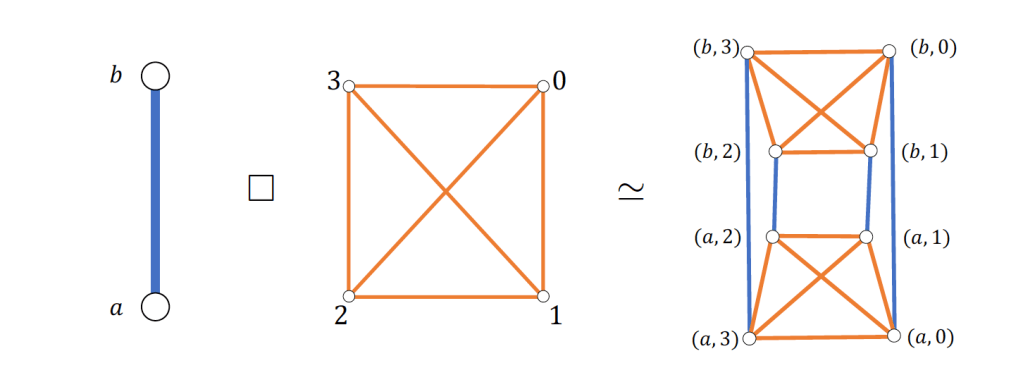
 of two graphs
  and
and  . (
. ( . Check that if
  -regular and
  -regular, then
  -regular.
  .
. 
 has a Hamilton decomposition.
  has a Hamilton decomposition.
 has a Hamilton decomposition.
  the graph which every Hamilton double-ray is isomorphic to.
 -distance graph, which has the integers as vertices, and an edge between two vertices
  iff
iff  .
. 

 :
: 
 , namely, a Hamilton decomposition is only possible if
  is even. What a relief it is then, that it is always possible if
 .
. 
 .
.  has a Hamilton decomposition, this would be a nice generalisation of Foregger’s and Aubert and Schneider’s results for finite graphs, either viewing
  as the lattice which already has a Hamilton decomposition, in which case Aubert and Schneider’s result would apply. If
  , in which case we simply have the lattice. Understanding any symmetry and pattern in the even case would be incredibly insightful for determining the odd case, but the construction becomes a bit too complex, and the pictures a bit too messy, that it would take a very careful hand to draw out the decomposition in a way we could wrap our heads around it. If you can manage to draw out the decomposition for
  , this would already be a more concrete example than anything I have managed to draw, and probably provide quite a valuable mental image of how to translate this to odd
  has all the right components for its own lovely symmetric solution, given that a decomposition would have 3 colours and the graph has an order 3 symmetry. Such a solution would provide its own insight into the other odd cases. So there is no reason a clever human brain couldn’t figure out a nice solution directly, perhaps inspired by the lattice decomposition. Alas, so far it seems that clever human brain might not be mine, but it might be yours!
You must be logged in to post a comment.