Sports – Page 2 – Jack Neubecker

Who Are the Best 3 Point Shooters?

April 29, 2016November 19, 2020Posted in Blog posts, NBA, NBA Statistics, SportsTagged JR Smith, Kevin Durant, Klay Thompson, NBA, Statistical Analysis, Steph Curry2 Comments

The 3 point shot is quickly becoming one of the most important plays to perfect on the offensive end. Coaches are beginning to realise the untapped potential of the long-range shot, and are starting to focus more of their offensive plays on getting good shooters open for 3 point shots, especially in the corner, which is becoming the most efficient play in basketball. Players are spending more time practicing the 3 point shot, and we’re seeing a lot more 4s and 5s working on the craft and floating around the perimeter, an almost unheard-of concept only a decade ago.

The league average for 3 point shots in the 2015-16 season was 35.4%, for an expected points per attempt of 1.062, vs the 2 point shot which is made at a league average of 49.1%, for expected points per shot of 0.982. The concept of Nash Equilibrium would suggest that there is an inefficiency in the shot selection of offenses, so we can only expect 3 point attempts to increase in the future. For those who don’t know, Nash Equilibrium is the idea that strategy selections in a game will eventually even out as better strategies are chosen more by players, and countered more often by their opponents. Applied to basketball, it suggests that offenses will continue to shoot more 3s, and defenses will focus more attention to 3s, until the expected points for 3s v 2s is the same, a state of equilibrium. For this reason, a good understanding of where these extra shots should come from, and who the best 3 point shooters are is an important factor to any decision maker on the basketball court.

Currently, there exist a handful of incomplete metrics for measuring the effectiveness of a 3 point shooter. 3 point percentage is nice, it gives you a good idea of the likelihood of one of their shots getting in the hoop, but as with any rate statistic, it comes with flaws. Most of them stem from the fact that shot selection and volume account for so much of the minute differences between good and great shooters. The best 3 point shooter of all time according to 3P% is Steve Kerr, who had a career rate of 45.4%. That’s great, but he only made an average of 0.8 3s per game. Contrast this with Steve Nash, who shot at a lower 42.8% but made 1.4 3s per game. Shooting at a great click is useful, but only if you use it. Having a high 3 point percentage is good, but it’s useless if you don’t use it as much as a player with a slightly lower percentage. So 3 point percentage can’t be our only metric for deciding 3 point effectiveness.

So if pure efficiency isn’t going to cut it, let’s try a volume stat instead. 3 Pointers per game should be a good measure. If 3 points are worth more than 2, the more made 3s the better, right? Wrong. If you go by 3P/G, LeBron James (1.4) is just as good of a 3 Point shooter as Steve Nash (1.4). But LeBron James’ career mark is a meagre 34.0%, as opposed to Steve Nash at a much better rate of 42.8%. Nash (3.2 3PA/G) takes 0.8 less attempts than LeBron (4.0 3PA/G) to make his 3s, so Nash is clearly a better shooter, and going purely off volume metrics isn’t going to be very helpful either. What is needed is a metric that effectively combines efficiency with a volume of efficiency.

The ultimate mark of a good 3 point shooter should be the amount of points that they score greater than the expected points off every possession which they end with a 3 point shot. Simplified, this is “points off threes subtract expected points”. The method for determining expected points off a possession was to take the average Offensive Rating for the league (Points/100 possessions) and divide by 100. This gives an expected points per possession for the 2015-16 season of 1.064. The formula for calculating how much better than 1.064 points per possession each 3 point shooter was, is 3*3P – 1.064*3PA. Now we have our formula, we can apply it to every player in the league to judge their 3 point effectiveness. All we need is a name — I started using 3PTEPA for 3PT Expected Points Added as a tip to some of Baseball’s divisive sabremetrics, and eventually settled on 3PTx, 3PT Expected. Plus, 3PTx sounds pretty edgy so I went with it.

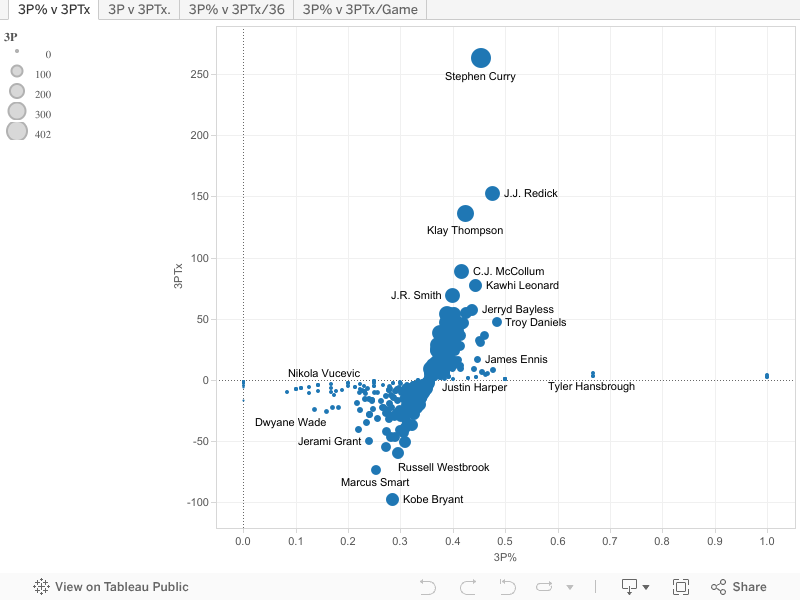
So let’s dive right in and have a look at the results when applied to player data for the 2015-16 season.

If your browser isn’t displaying the embedded graphs above, click here to view the interactive graphs on tableau.com. Scroll over data points for information about that player. To zoom in on a particular area, highlight that area, then hold the mouse over it until a box appears, and click “Keep Only”. Use the tabs up the top to switch between graphs.

First, let’s simply look at 3PTx. To nobody’s surprise, Steph Curry is head and shoulders above the rest of the cohort, adding 263.3 points this season on 3 point shooting alone. More than 100 points behind we have our second tier of shooters, Klay Thompson and JJ Redick, followed by our third tier of CJ McCollum, Kawhi Leonard and JR Smith.

At the other end of the graph, we can see which shooters have been hurting their team with every 3 point attempt this season. At the bottom, with -97.9 points is Kobe Bryant. It’s no surprise, because only Kobe has the respect to keep chucking up low percentage shots and not get benched, and this is a single-season number we may not see again for a long time. Zooming in on the bottom end shows us some of the other players with the worst shooting seasons, including names like Marcus Smart, Russell Westbrook, Corey Brewer, Jerami Grant and Kentavious Caldwell-Pope all garnering scores below -50.

So what can we learn about this graph in general? Well, for those at the very top of the graph, shoot more. For those at the very bottom, shoot less. But for the majority of players clumped into the middle of the graph, it’s a little more complicated. In the middle, it’s best to split our graph along a diagonal line like so:

For those who fall above and to the left of the line, they can attribute their negative score mostly to just being bad shooters. For those who fall below and to the right of the line, their score can be attributed primarily to putting up a volume of bad shots. Additionally, for players who, over the entire season, have a score of -20 or better, it’s worth considering that those attempts might not be that much of a negative influence. For example, players like John Wall or Gordon Hayward, who had season 3PTx scores of -4.0 and -7.2 respectively. Part of the 3 point shot is forcing the defense to respect you on the perimeter. If Wall or Hayward had shot considerably less from 3 this season, they probably would have a harder time getting to the rack as opponents sag off, as well as spreading the floor less for their team mates. So sometimes with players you need to take the good with the bad. However, if Wall had chosen not to take only 4 extra attempts this season, he would have broken even, so players with negative scores should still learn from that statistic when deciding to force a possibly ill-advised 3 point shot.

It’s very interesting to look at where a lot of players lie on this graph, some of the most interesting ones I’ll note here. Marvin Williams is on the same level of shooters as players like Kyle Lowry, Kevin Durant, and Kyle Korver, right at the top of the main pack, proving once again how much of an underrated season he’s having for the Hornets. Players considered by most to be good shooters who had a terrible season: Monta Ellis (-39.0), Nik Stauskas (-27.8), Danny Green (-23.3) and Paul Pierce (-32.5). Also, more proof of how poor LeBron James’ shooting has become this season, costing his team 39.0 points on the 3 ball for only 87 makes on the season. Stop shooting 3s LeBron. Please. Continuing on the stars who shoot 3s too much, Carmelo Anthony (-14.8) hasn’t had a great season. There are also a lot of players considered to be stretch fours or shooting bigs that find themselves with negative scores. Serge Ibaka (-15.8), Kristaps Porzingas (-15.6), Al Horford (-8.4) some of the biggest names, however as discussed before, the floor-stretching they provide may be worth the lost points.

Finally, it’s worth noting that the watershed mark for good or bad 3 point shooting is right around the 35% to 36% mark, which seems to gel with the consensus opinion around the league, which shows that our perception of 3 point shooters is reasonably consistent with game theory.

The 3PTx statistic provides a good look at the overall impact of a player’s 3 point shooting on the season, but a per-shot perspective might give us a better look at which players cause the most damage with every shot, and which players can afford to take more threes to up their efficiency. The next tab on tableau.com displays 3PTx. plotted on total 3 pointers taken. 3PTx. is simply calculated by 3PTx divided by 3 Pointers attempted.

Simply looking at where players fall along a ladder of 3PTx. scores would be interesting enough, but fleshing out the points by looking at total 3s gives us a good idea of how much of a player’s 3PTx. score can be attributed to low sample size, and if so, how many more shots they can afford to take.

Here, we get a better look at some players who have been neglected on the 3 point line. The players we see at the top of the graph with only a handful of attempts can obviously be ignored, because their percentages came off a very small sample size. This metric suffers from a lot of the same flaws as simple 3PT%, but it does benefit from at least giving a reference point of whether a given rate is a good or bad percentage.

For players who find themselves below the 0 3PTx. line, it’s better for them to additionally be found with less 3 pointers made, because the more that come off a bad rate, the more a player is hurting their team. For those above the line, they should want to find themselves with as many 3 pointers made as possible, because each attempt is good for the team. Information about individual players can’t be explored as much as with the previous graph.

The third graph plots 3PTx/36, a measure of how many points a player adds through 3 pointers per 36 minutes of court time. Steph Curry finds himself highest amongst high volume players, to no surprise, but we also find a few players around his range whose value on the court may have been overlooked when it comes to the 3 pointer. Steve Novak and Troy Daniels stand out the most, but obviously these players have bigger flaws in their game which force coaches to sit them, despite their good 3 point shooting. This measure is best for judging players in the middle of the pack and comparing similar players, just like other /36 statistics.

The final graph plots 3PTx/Game, another metric which provides a good equaliser, however this stat is more effective for multi-season comparison, or contextualising a number. This graph will be much more interesting when comparing historical players, whereas for single-season data it looks almost exactly the same as the first graph which simply plots 3PTx.

It should be seen from this rudimentary exploration of the results how effective 3PTx is as a measure of 3 point shooting. This statistic would be a good advanced stat to use in analysis of a player’s shooting, and provides a single number on the level of box-plus-minus or Win Shares which immediately allows one to make conclusions about whether a player’s shooting is a negative or a positive. In my next article, I will be applying this data to historical 3 point shooters and subsequently judging the best and worst players of all time when it comes to long-range shooting. Further down the road, I am looking to try and implement a similar strategy to a player’s entire scoring output, to discover who the best all around scorers of all time are. But until then, enjoy the use of this metric for analysing 3 point shooters. Contact me if you’ve got any suggestions for how this metric could be improved, or your general thoughts.

statistics provided by Basketball Reference
Graphs provided by Tableau.com
Read about how this statistic applies to all-time 3 point shooters here
twitter: @jackneubecker
email: pointforwardpod@gmail.com
An Article by Jack Neubecker

An Honest Reflection on Tanking

April 17, 2016April 5, 2022Posted in Blog posts, Historical Discussion, NBA, NBA Draft, NBA StatisticsTagged Basketball, Draft, History, NBA, NBA Draft, VORP1 Comment

How Effective is Tanking?

In the wake of Sam Hinkie’s resignation as GM of the Philadelphia 76ers, there has been a lot of reflection about the effectiveness of his aggressive strategy. First of all, this is pretty unfair on Hinkie, because the job isn’t done yet – it’s about now that the 76ers land themselves a star in Brandon Ingram or Ben Simmons, and use that to lure a free agent and start to climb their way back to the top, but that’s just an aside. As a result of this, a lot of subsequent discussion has followed about the effectiveness of tanking in general. The most oft-used strategy for breaking this down is a lot of anecdotal, team-by-team evidence. Analysts will point to the Warriors as an example of how to win a championship without a number one pick, and their debating opponents will immediately fire back with the half-dozen championships won by number 1 picks in LeBron and Duncan in recent NBA history. After listening to this debate from both sides of the argument for a few days, I started brooding and pondering, and eventually decided I should investigate with some rigorous statistical analysis that removes the element of ambiguity.

Before I get into the research I conducted, I’ll just lay some groundwork for this discussion. Right off the bat, I’ll ask the question: “Which teams haven’t been bad in the past 8 years?” – the answer is a list of 6 teams, give or take: the Spurs, Rockets, Bulls, Mavs, Heat and Blazers. That’s 6 out of 30 teams in the NBA, so when someone says “x team bottomed out that year, got this player and is now a contender” the overwhelming likelihood is that any team has bottomed out. It’s not fair to point out that the Clippers sucked and got Griffin and now they’re good, when in reality every team has been bad at least once. Also the Clippers were terrible for a long time, a fact I know from experience, so eventually they were going to land a star. It fails to consider all the teams that bottomed out and haven’t picked up any talent to lift them into contending status (think Kings, Suns, Knicks, Pelicans, Timberwolves, Magic). So let’s look at this topic analytically, and develop some measure of a player’s likelihood of winning a championship.

PART 1

The first relationship I thought I should explore is draft position vs win shares. If tanking works, we should see a lot of the win shares going in the first handful of picks. I thought it would be important to set up my timeframe beforehand, because everyone’s favourite activity is taking a statistic and playing with the specifics until it suits your point of view. I chose the 1994 draft as the earliest draft to consider, because it was the first one to look like the draft we have today, with a distributed lottery and (almost) 30 teams. It also gives a good 22 year timespan for any anomalies to be ironed out, there’s nothing worse than a small sample size. It’s also the year of the Glenn Robinson draft, so I wasn’t just going to cut him out to favour an anti-tanking stance, and it’s 1 year before the draft of Kevin Garnett, the earliest active player drafted.

I chose win shares as the statistic as it is the best advanced stat out there for success of a player. The player with the most win shares is Kareem Abdul-Jabbar, because he created a lot of wins over a long period of time. Jordan is 4th due to his career being shorter than Wilt and Malone before him, but his win shares per 48 minutes is the best of all time. The career win shares list can be found here <http://www.basketball-reference.com/leaders/ws_career.html> and I think you’ll agree it’s a good indicator of a player’s likelihood to win championships, seeing as winning is the point of basketball. You might be put off by the fact that MJ isn’t first, but if you want to maximise championships, longevity is a very important factor. You might also point to players like Chris Paul or Charles Barkley, who have plenty of win shares but no championships. Maybe there’s something to that, and pure win shares isn’t everything, but the most likely explanation for that is just plain bad luck, given how difficult it is to win a championship each year, even for the best team.

I took the win shares stat for every player drafted since 1994, and slotted them into draft position. I then graphed the total win shares from each draft spot since 1994 and got this:

Click here for a high quality version of the above graph

Clearly, you can see that the win shares are pushed towards the front of the draft. Highlighting the top 10 win share contributors since 1994 shows that, with the exception of Kobe Bryant, they all went in the first 10 picks. The most important thing to take from this graph is that the advantage of having the number 1 pick isn’t that great, the dropoff from 1 to 5 isn’t great, and neither is it from 1 to 10. The other important thing to learn is that a lot of wins go well after the lottery. You’re by no means missing out of you don’t have a high lottery pick.

Obviously there is a lot of noise in this graph, and another way of looking at this data helps eliminate the bumpiness. This graph takes the cumulative total of win shares taken after a certain pick. Think of it as the amount of win shares already taken if you pick at a certain position.

You can clearly see from this graph that a quarter of the wins available in a draft will go within the first 5 picks, and the next quarter will go in picks 6-12. Almost 80% of the wins will be gone by the end of the first round, so about 30% of the win shares are still available to non-lottery teams every draft.

It’s also interesting to look at the median win shares for each pick. Median is the middle score in a set, so this value is useful for eliminating players who far exceed expectations or are complete busts, and is probably a better indicator of the most likely player you would expect to receive from a specific spot.

It backs up the observation that you’ll find the best players at the top of the draft, but there’s still some nice players to be found at the end of the lottery and smattered throughout the end of the first round. Interestingly enough, your median 3rd pick will contribute more wins than your median 1st pick. If I were to wager a guess, I’d say that this is because in addition to generational talent being taken at #1, you also get a lot of boom or bust players that eventually bust, think Michael Olowokandi, Kwame Brown, Andrea Bargnani or Greg Oden.

So, what can we learn from the relationship between win shares and draft pick?

– the best players generally go at the top of the draft (it’s comforting to know that NBA GMs aren’t just rolling dice to determine their pick)

– there are plenty of wins to be found outside of the number 1 pick, and still plenty outside of a top 5 pick.

– you won’t find a good player with the 6th pick, ever. Seriously, if anyone can suggest a reason why the 6th pick is so significantly worse than all the surrounding picks, let me know, because it’s so much worse that it almost can’t be chance.

This relationship would suggest that if you can get the number 1 pick, that’s the best place to find a superstar, and settling for the 2-5 pick isn’t a bad substitute either. That being said, there are plenty of players to be found outside of the top 5 picks. So after one relationship, I’d say it’s about 55/45 in favour of tanking. But this relationship is by no means the end of the story.

While this is a good indicator of where the talent comes from in a draft, maybe it’s not the best indicator of championships, because as everyone knows, you need all-stars to win championships, there’s only 5 players on the court so your talent needs to be condensed to win championships. So the logical next step is to look at where championships come from.

PART 2

This is a much harder relationship to investigate than it might initially seem, for a few reasons. First of all, simply finding out how many championships a player has won isn’t as easy as it might seem. It’s not one of the key stats at the top of a player profile, and it’s certainly not a column in a draft summary table. Even if it were easily sourced, that wouldn’t be the most practical way to do things, because not all rings are earned evenly. Purely by championships, Robert Horry is a better player than Dirk Nowitzki, but not a single person who knows how to pronounce Nowitzki would take Horry over Dirk. Therefore, we need a better measure of championships won by a player at a certain draft position.

My solution was to partition each championship into weighted shares based on each player’s contribution to the team that season. The best way to split up players was by win shares, so every player on the roster of a championship team was credited with a championship share. Take LeBron, who had 14.5 win shares in the 2011-12 season, out of the heat’s combined 48.1 win shares. LeBron is credited with 14.5/48.1 championships for that season. This gives most of the credit to the key players on the roster without neglecting role players who are nevertheless essential to a championship team. The timespan was again any player drafted since 1994.

The result of breaking up these championship shares by pick position looks like so:

What you get is a more noisy version of the graph we produced by looking at win shares. In one aspect that’s good, because it shows that win shares was probably a good indicator of likelihood to win a championship. But in another aspect, it makes it difficult to try and gain any insight from the data. Let’s start with the bumps. I would say that there are 5 pick positions which can be called bumps in the data. Pick 1, 5, 13, 28 and 57. Pick 1 can be attributed to two players, Tim Duncan and LeBron James, with sprinklings of Glenn Robinson and Andrew Bogut. Pick 5 is a mix of Dwyane Wade, Ray Allen and Kevin Garnett. Pick 13, 28 and 57 can be attributed almost solely to Kobe Bryant, Tony Parker and Manu Ginobili respectively. If we take into account these factors, we can see a similar trend to the previous graph, that a lot of the talent goes at the top of the draft, but there’s still plenty left by the end of the lottery and even an entire half a championship left at the 57th pick.

Looking at the cumulative total tells the same story, where we see roughly half of the championships are taken by halfway through the first round, and the rest is spread out over the following round and a half. Taking a look at the players responsible for the bumps, it needs to be noted that, with the exception of LeBron James, Kevin Garnett and Ray Allen, all of these players were drafted to excellent teams that were already title contenders. The three exceptions all moved to other teams in pursuit of a championship, and earned their chips there.

So the lesson to be learnt from this graph is that nba championships are as much a product of the team you are drafted to as your inherent ability as a basketball player. This would suggest that having a good team environment is essential to growing your talents as a rookie in the NBA. Would Manu Ginobili have created 0.5 championships in his career and won 4 in total were he to have been drafted 1 pick earlier to the Warriors? Almost certainly not, without Pop and Duncan he probably would never have won a title. Would Kobe Bryant have earned an entire championship share and 5 rings in total were he to have not been traded on the day of the trade to the Lakers and instead played for the Hornets? Full respect for Kobe, but probably not without Shaq and Phil Jackson and later Pau Gasol.

So the conclusion from this relationship is that the make-up and quality of the team is critical to a player’s success. This skews the argument heavily in favour of an anti-tanking stance, probably at about 75-25 in favour of not tanking. But this data was based off an admittedly small sample size, there’s another piece of analysis that would be very helpful to evaluate effectiveness of tanking.

PART 3

One way of taking a broader look at the effectiveness of tanking is to stop looking at all of the individual players taken at specific spots, which can be affected by single players who just buck the trend, and instead look at the future success of teams who pick at particular spots. So for the next analytical look at tanking, I charted pick position against the subsequent success of the team for the next 8 years. I chose 8 years because it is a long time, about the length of a player’s first two contracts, and a good length of tenure for a GM to turn around a failing franchise. So take the 1994 draft, where the Bucks picked first. I took their average win percentage for the next 8 years and put that into the number 1 pick data. The next year, the Warriors had the number 1 pick, so I took their win percentage for the next 8 years and added that to the number 1 pick data. After repeating this for every first round pick in the NBA since 1994, I developed a graph of team pick position vs subsequent team success, which looked like so:

(aside: I removed the second pick for a team that had multiple first round picks, as I didn’t want the data to be affected by duplication)

The only conclusion that can be drawn from this graph is that it makes almost no difference, the pick positions that perform the worst aren’t that far displaced from the teams that perform the best, excluding some outliers. This is a good sign for the NBA in general, since the point of the draft from a league perspective is to level the playing field, so it’s good that everyone experiences regression to the mean. It’s also worth observing that picking in the middle of the draft, in the so-called no-man’s-land of the NBA, appears to net you a better win% over time than any of the picks further up the draft, with the exception of the number 1 pick.

Additionally, there are no better results than if you can get yourself into a pick right at the end of the draft by being a pretty good team in the first place. So the conclusion here is the better you are, the better your win% will be in the future, unless you can land the #1 pick in the draft. If you tank and don’t get the number 1, you’ll end up in that 2-5 zone which results in the worst records of all picks. However, thanks to the lottery, the odds of getting the number 1 pick if you’re the worst team in the league are only 25%. This more than eliminates the incentive to get the number 1 pick, because it’s not automatic, even if you do suck, and if you win the lottery for second place you’re just stuck in a terrible place anyway.

The good thing about this model is that it isn’t biased by all of the randomness associated with players once they enter the league. This model accounts for the fact that a player might go searching for a new team in free agency, or that they get injured, and account for the fact that to get the number 1 pick, you need to be a bad team to begin with. When factoring in the effectiveness of tanking, you need to consider the fact that if you do land a superstar, they might not want to play for you (see LeBron). And look at the blip at the number 1 pick, it still doesn’t reach above the .500 mark! The only reason that bar is any higher than the ones around it is because of a few guys.

There’s one team that won 70% of their games after the number 1 pick – the spurs (if you’ve got Gregg Popovich as your coach, you can do it. Otherwise, no chance), and only 4 teams that won more that 52% of their games after the number 1 pick. Out of 14 drafts considered, there’s a 4 in 14 chance that you’ll get a player that turns your franchise around. So if you can be so bad that you’re the worst team in the league, you have a 25% chance of getting the number 1 pick (the only one that’s worth getting as can be seen from this graph). And after that, you’ve still only got a 28.6% (4 in 14) chance of that #1 pick being a player that will turn your franchise around. So if you’re the worst team in the league at the end of a given season there’s a 7.1% chance that you’ll become a +.500 team as a result. In other words, don’t bother tanking.

After Part 3, let’s say I’m now fairly in favour of not tanking.

PART 4

Regardless, let’s soldier on further and see if we can dive deeper and gather a defense of tanking! That last relationship still doesn’t truly get to the roots of the issue, because win% is one thing, but the whole point of tanking is to win The Larry O’Brien Trophy, the true mark of a team’s success. (aside: if it means being like the 76ers for 3 years, and being a disgrace to the NBA and compromising the integrity of the league and turning people off being fans of your team, I don’t think it’s worth it to win one trophy, vs being a consistently respectable organisation) So let’s see if we can go one step further and instead look at the subsequent championships after picking at a certain pick. Luckily for me, it only took subbing in the championship winner each year to my spreadsheet instead of wins to get me that data. So let’s have a look at exactly the same process but chips instead of wins.

That’s pretty depressing for anyone with the number 1 pick, let’s be honest. Oh and by the way, if you’re still saying “but it’s still be best of a lot of inefficient strategies” if I take away 1 draft, the 1997 draft that saw Tim Duncan go to the Spurs, there is not a single team that has turned a number 1 pick into a championship in the 8 years following their selection. None. So tanking: not looking good.

Okay, this sample size isn’t huge, there have only been about 20 championships in this whole time frame, so let’s see if we can pad all the numbers up a little bit, flesh things out. Conference titles. Everyone agrees if you make it to the dance you’re in with a good shot.

Well, that hasn’t helped the case of the number 1 pick at all. Again, if you take out Tim Duncan, that line goes down some more and it’s almost no better than the next few picks all after it. So the case for the number 1 pick being a boom or bust strategy that could land you a championship is in a shambles.

CONCLUSION

So, after looking at all of those independent pieces of data and formulating a conclusion, I’ll enunciate them here. It’s pretty clear that tanking has worked once, the 1997 draft to select Tim Duncan. One time. Other times, it’s been effective at picking up stars, like LeBron James. But still no championships. So in the last 20 years, tanking has worked once, and you know why it worked? Because a humble, low-ego, super-talented player entered the league onto the roster of one of the best coaches in NBA history, put his head down and learnt and practiced and grew into one of the best power forwards of all time. He also landed on a roster that had some really good pieces and a former number 1 pick already there.

When the spurs got Duncan, it was a 1 time deal, they were bad for a single year thanks to injuries, lucked into Duncan and never looked back. So what we can learn from the one time tanking worked is not that tanking works, but instead that if you’re one of the best coaches in NBA history, you can make it work. But what of players like Kobe Bryant, Paul Pierce, Kevin Garnett? Well it’s pretty clear that the reason they were successful is because of a smart GM who saw their talent and landed an absolute gem later in the draft. We saw it work with the Spurs twice, when they drafted Tony Parker and Manu Ginobili with the 28th and 57th picks respectively in their own draft classes. Kobe and Pierce were also drafted to historically good franchises, and Garnett won his titles with one of those historic franchises.

I think the biggest flaw in thinking for those who expound tanking is a big assumption about the talent coming out of a draft. They assume that LeBron was a board-eating, dime-dropping, muscle-machine MVP when he was drafted, but in fact it took him years to develop the skills to be the player he is today. What he was, was a hard worker and hyper-dedicated. Duncan wasn’t drafted as one of the most skillful, graceful post players of all time. He was a hard worker, and extremely humble. See the same for every other transcendental talent, they got where they are because of hard work that continued into the NBA. If Duncan were to be drafted to the Sixers in this year’s draft as the lanky 21 year old he was in 1997 – without the help of David Robinson and Gregg Popovich – he wouldn’t win 5 titles. Straight up, he wouldn’t. Coaches and GMs win Championships. Let me phrase that another way, good teams win Championships. Good teams don’t lose on purpose. Don’t lose on purpose. Don’t tank.

You can look at the spreadsheets I used for this data here
Statistics were sourced from Basketball-Reference
An Article by Jack Neubecker

2016 NBA Playoff Probability Model

April 16, 2016November 19, 2020Posted in Blog posts, NBA, NBA Playoffs, NBA Statistics, Sports1 Comment

Hello again basketball fans,

It’s that time of year again, everybody is getting excited for the start of the NBA Playoffs, the thing we’ve all been waiting for. Last year, I debuted my playoff probability model for determining the likely outcome of specific games and applying it to a playoff series and the whole playoffs. If you would like to read up on the finer points of how it works, you can do so here. This article, however, will focus primarily on interpreting the results of this year’s data.

Absolute Model

While it is a bit of a bastardisation of statistics, the absolute model is always a good place to start when it comes to the playoffs. Figuring out which teams are chalk and the single most likely path to the NBA Championship is always interesting. It doesn’t allow for much flexibility, but let’s have a look at how things are most likely to fall into place.

WEST
1	GOLDEN STATE	0.94471087992732	4
8	HOUSTON	0.0552891200726802	1

4	CLIPPERS	0.722588694531871	4
5	PORTLAND	0.277411305468129	1

2	SAN ANTONIO	0.973154022027252	4
7	MEMPHIS	0.0268459779727475	0

3	OKLAHOMA CITY	0.865586033788547	4
6	DALLAS	0.134413966211453	1

EAST
1	CLEVELAND	0.781272507835133	4
8	DETROIT	0.218727492164867	1

4	ATLANTA	0.707338094725949	4
5	BOSTON	0.292661905274051	1

2	TORONTO	0.695089397073879	4
7	INDIANA	0.304910602926121	1

3	MIAMI	0.483887327493713	2
6	CHARLOTTE	0.516112672506287	4

The first result is not too much a surprise to anybody, the Warriors should smash the Rockets in the first round. The model predicts Houston to take one game, probably as a result of the fact that the Warriors only have a 66.6% chance of winning a game played in Houston. (I know! only 66% on the road) This is a fair thing to assume seeing as the Rockets have the all-star talent to compete against the Warriors and will at least give them a run for their money. That being said, this series is not in doubt. For the Clippers against the Trailblazers, the series is not the foregone conclusion of the 1v8 matchup, but the most likely end result is much the same, a 4-1 series victory.

San Antonio vs Memphis promises to be more of a whitewash than the Warriors’ first round matchup, with the rare occurrence of the model actually predicting a 4-0 clean sweep. This is somewhat to do with the fact that the Grizzlies have been rolling out replacement level players for months to try and plug holes in an injury-ravaged roster. The Spurs are 73.3% favourites in Memphis, so a 4-0 victory is quite likely. Finally, Oklahoma City vs Dallas seems to be a pretty predictable series similar to the rest. I’m confident the Mavericks can take one game in the series, given they have a 38.8% of winning a game played in Dallas. These two teams have had interesting playoff matchups in the past, maybe we can hope for another interesting matchup this series. However, that’s unlikely, and I’d have to put the over-under on games won by the losing team at 3.5.

In the East there at least promise to be some interesting matchups. Cleveland vs Detroit looks to be a pretty predictable conclusion. However personally, I think it will be a frisky matchup because of the contrast between the pampered, unappreciative Cavaliers who whinge and complain all the way to the finals, and the unimpeachable enthusiasm of the happy-go-lucky Pistons. The 4v5 matchup between Atlanta and Boston doesn’t appear to be the close, exciting matchup it might first seem. This is most likely because of Atlanta’s road strength resulting in a 56.1% chance of winning a game played in Boston. While the single most likely result is a 4-1 series, the over-under should be put at 6 games in the series, as the 50th percentile of probability would result in a 4-2 series. And just as much of a possibility to consider in a 4-3 series, which at that point could go either way.

Toronto vs Indiana appears to be a pretty uninteresting matchup, with a 69.5% chance of Toronto winning the series. It’s most likely that the Pacers will take at least one game given their strength at home. Miami vs Charlotte looks to be the most interesting series in the first round, with the Hornets pulling off the upset over the 3rd seed in a very close series. There’s almost nothing between these two sides, but the biggest strength is the Hornet’s 64% chance of winning a game played in Charlotte, and that looks to be the deciding factor.

Second Round

GOLDEN STATE	0.852616270754272	4
CLIPPERS	0.147383729245728	1

SAN ANTONIO	0.697841551815112	4
OKLAHOMA CITY	0.302158448184888	1

CLEVELAND	0.644809408549719	4
ATLANTA	0.355190591450281	1

TORONTO	0.645999031198189	4
CHARLOTTE	0.354000968801811	3

The Golden State vs Clippers matchup looks a lot like those of the first round matchups, a disappointing sight for a Clippers fan such as myself. The Warriors have a 56.4% of winning in Los Angeles, so the Clippers have the chance to at least home home court, but this series will most likely be a 4-1 series, maybe 4-2. San Antonio vs Oklahoma City promises to be a more exciting matchup, with a 70% chance of the Spurs advancing thanks to their home dominance. While the model says the single most likely result is a 4-1 series, the 50th percentile occurs at a 4-2 series win for the Spurs, so there’s at least something in this matchup.

In the East, Cleveland vs Atlanta looks to be a reasonably close series, and it very much resembles the Spurs vs Thunder matchup from above, both in home court strength and likely result. And Toronto vs Charlotte looks to be a really exciting series, with the result being Toronto winning in a game 7.

Conference Finals

GOLDEN STATE	0.567784275220779	4
SAN ANTONIO	0.432215724779221	3

CLEVELAND	0.60235080881409	4
TORONTO	0.39764919118591	3

The Golden State vs San Antonio matchup is what we’ve all been waiting for. A really close matchup that ends up being decided purely on Golden State’s home court advantage in the 7th game of the series. The Warriors have a 62.5% chance of winning in Oracle Arena, and the Spurs have a 59.6% chance of winning in the AT&T Center. This series is going to be awesome, and an upset win on the road will most likely be the ultimate decider here.

In the East, a less close but probably similarly exciting matchup is going to go down between Cleveland and Toronto. The deciding factor is the 50/50 nature of games played in Toronto. If the Raptors are to pull off an upset of the 1 seed, they’ll need to hold home court and pull off the 41.5% chance of beating the Cavaliers at home.

Finals

GOLDEN STATE	0.779957658270466	4
CLEVELAND	0.220042341729534	1

This looks to be an almost repeat of the same finals matchup we saw last year:

GOLDEN STATE	CLEVELAND
0.77231315859749	0.22768684140251
4-1 WIN

Almost exactly the same. Golden State’s relative increase in dominance has been matched by Cleveland’s increase in attaining the top seed in the East. We’ll probably see almost exactly the same result as well, a 4-1 win to the Warriors. Why am I not surprised?

Probabilistic Model

Now for the real deal, the model that accounts for every single possibility in the fall out of the playoffs. Read up on last year’s article for a more detailed explanation of how it works, but here I’ll go through the predicted results for every team.

		WIN CONFERENCE SEMIS
1	GOLDEN STATE	0.831564662237668
2	SAN ANTONIO	0.71171406663822
1	CLEVELAND	0.611241117020462
2	TORONTO	0.47246401788129
3	OKLAHOMA CITY	0.275855523155884
6	CHARLOTTE	0.217613191031987
4	ATLANTA	0.206032505330248
3	MIAMI	0.172783791336251
7	INDIANA	0.137138999750471
4	CLIPPERS	0.129562772628827
5	BOSTON	0.0993505861405786
8	DETROIT	0.083375791508711
5	PORTLAND	0.0214138651858404
6	HOUSTON	0.017458699947665
7	DALLAS	0.00915097052567799
8	MEMPHIS	0.00327943968021826

The odds of winning in the second round of the playoffs and making it to the conference finals don’t come with any surprises for the top 5 teams, and these are the teams which are considered to be the contenders this post-season. The first surprise is the Hornets, who jump above heat thanks to the likelihood of a first round upset over Miami, and their subsequent relatively good matchup against the Raptors. Atlanta jumps above the Heat as well, thanks to the fact that they have an easier matchup in the first round. The biggest surprise is how low the Clippers are, but this is almost entirely because of their impending Warriors matchup in the conference semi-finals. The only interesting things at the bottom of the list are the high odds for Detroit compared with the 5-8 seeds in the West. This is most likely because the bottom seeded Western Conference teams all have very difficult matchups in the first and second round thanks to the juggernaut top seeded teams.

		CONFERENCE CHAMPION
1	GOLDEN STATE	0.509894738843795
1	CLEVELAND	0.402470870514094
2	SAN ANTONIO	0.35934556145901
2	TORONTO	0.236511454787246
4	ATLANTA	0.105711934024377
3	OKLAHOMA CITY	0.0991444531961068
6	CHARLOTTE	0.091155111322623
3	MIAMI	0.0592052077624748
7	INDIANA	0.046857460596964
5	BOSTON	0.0304294701923865
8	DETROIT	0.0276584907998341
4	CLIPPERS	0.027156423486168
5	PORTLAND	0.00185687769931837
6	HOUSTON	0.00159832431602761
7	DALLAS	0.000819347027150694
8	MEMPHIS	0.000184273972424295

In the probabilities for the eventual conference champions, we see much of the same, with the top 2 seeds 1st and second respectively in their conferences for likelihood to make the Finals. We don’t see any of the anomalies of the Clippers/Spurs in last year’s model, thanks to the seeding being a lot more sensical. Atlanta, Oklahoma City and Charlotte each have about a 10% chance of making the finals, and then the rest are all under 6%. The 4-8 seeds in the west are all shunted to the bottom of the list amazingly, showing just how dominant the top 3 seeds in the Western Conference are.

		CHAMPION
1	GOLDEN STATE	0.430867495224729
2	SAN ANTONIO	0.30034047968401
1	CLEVELAND	0.104910022252147
3	OKLAHOMA CITY	0.0649931197327366
2	TORONTO	0.0436546468759919
6	CHARLOTTE	0.0147048159767159
4	CLIPPERS	0.01321875494538
4	ATLANTA	0.00948918037371775
3	MIAMI	0.00568379816142752
7	INDIANA	0.00472936681828004
5	BOSTON	0.00364924486409851
8	DETROIT	0.00259974086000893
5	PORTLAND	0.000484601036206965
6	HOUSTON	0.000448137088936561
7	DALLAS	0.000196654101541757
8	MEMPHIS	0.0000299420040720599

We see here that Golden state is the favourite with a 43.1% chance of winning the Championship. This is down from last year’s odds despite their dominant season thanks to one factor: The Spurs. We see the Spurs second with a 30.0% chance of Pop bringing home a 6th title, followed by a 10.5% chance of Cleveland breaking its 3-team championship curse after 52 years. Oklahoma City and Toronto are the only two other teams with considerable chances, at 6.5% and 4.4% respectively. We see the Clippers take a rise thanks to the fact that if, by some chance, they do make it to the finals, they would be a good chance of winning against their opponent.

The Warriors are going to have a tougher time defending their title than you would expect from a team that only lost 9 games in the entire season, thanks to another historically good team nested in their own conference. For that reason, I can’t feel comfortable making any wagers on so few losses like I did with my co-host last year, but it will make for much more exciting playoffs. A 7 game series between the Warriors and Spurs is going to be absolutely amazing, and we have about a 60% chance of seeing these two playing each other in the Conference Finals. I can’t wait, these Playoffs are going to be great.

If you would like to see a copy of the data and process used for these probabilities, you can find a numbers file here, an excel file without interactive pop-ups here.
Box scores used for analysis were sourced from Basketball-Reference
Last year’s article explaining the model can be found here
Based on previous advanced analytics work by Dean Oliver <http://www.rawbw.com/~deano/articles/BellCurve.html>, Brian Burke <http://archive.advancedfootballanalytics.com/2009/03/comparitive-modeling-hockey-as-poisson_12.html>
Find a podcast where I explain the model in depth here
An Article by Jack Neubecker

Playoff Probability — Using Standard Deviation to Predict Playoff Outcomes

April 18, 2015November 19, 2020Posted in Blog posts, NBA, NBA Playoffs, NBA Statistics, Sports3 Comments

Introduction

This report will demonstrate how I used Standard Deviation, team offence and defence to produce an accurate model for predicting the results of NBA playoff series, and subsequently probabilities for the entire playoffs. This work builds on similar work in basketball and ice hockey, and adding my own previous work in playoff series probability and standard deviation. Predictions are then subsequently made about the results of the NBA playoffs and an overall NBA champion is predicted. Limitations of the model and possible ways of improving it are then discussed. The spreadsheet used can be found as a numbers document here, as an excel spreadsheet (unsure about formatting) here, and as a pdf (view only) here. You can also listen to a podcast where I walk through and explain the workings of the model here

Developing the Model

This analysis is based on an article published by basketball researcher Dean Oliver and has been built on based on the principles discussed in this article. Oliver has taken the scoring average and standard deviation of a team, and compared it to the defensive average and standard deviation of that team and calculated how many wins they should have earned. By using a normal distribution Oliver has calculated the probability of a team scoring a particular amount of points in one game, and compared that to the probability of their opponent scoring more points than them. This can then be boiled down into one number that produces the overall win probability for a team on any given night.

The one problem in this model is that it does not account for a team playing up or down to the level of their competition, for example garbage time. This allows one team to close the margin of victory without the result ever being in doubt. But this effect is small, so it is reasonable to exclude it. What is relevant to my research from this article is that one can extend this to individual game results. If the scoring average and standard deviation of two teams can be calculated, principles from Oliver’s paper can be used to determine the probability of either team winning.

Alone, this model does not account for the effect of each team’s defence, in order to do so, I used the same technique as is used in the following article . Simply adjust the average for each team’s scoring output based on their opponent’s defence compared to the league mean. A team with above average defence that holds their opponent to on average 97 points (compared to league average 100) means they would have a defensive impact of 3 points, so 3 points would be subtracted from their opponent’s scoring average.

From these calculations, Adjusted offensive average and standard deviation can be determined, and these are the figures used to calculate the win probability for either team. The next step is to account for home-court advantage. By collating the scoring outputs of every playoff team and separating home performances and away performances, one can easy break down the effect of HCA on every team. By doing this, and treating Team A on the road as a separate entity to Team A at home, the win probability for a team at home and away can be calculated. For example, in a series between Boston and Cleveland, Boston at home is pitted against Cleveland away, and alternately, Cleveland at home is pitted against Boston away. From this, the effective win probability for every game of a playoff series can be calculated.

The formulae and techniques used can be seen in the spreadsheet in the sheet named “Bell Curve Analysis”. After all of those stats have been collated, probabilities can be calculated for a game against any two teams, accounting for home or away. Once these WPs have been calculated for both scenarios, a model can be constructed to calculate how these would play out over a 7-game series in the format HH-AA-H-A-H (other formats could be used but this is the model for all current NBA playoff series).

The calculations are a simple weighted probability tree, which can be found on the sheet named “7 Game Series”. This model has various benefits, namely it properly accounts for the effect of the change in HCA throughout a series, and it also provides a good estimate of what the exact result for the series will be (how many games will be played). The one drawback of the model is that it will almost never predict a 4-0 series sweep, because the 4-1 result will almost always be more likely as the favourite will be back on their home court.

However this is not as much of a limitation as previously thought, as it makes sense to think that 4-1 is almost always the more likely result, 4-0 is a surprise no matter the quality difference of the two teams. The spreadsheet has also been modified for ease of making these series calculations. On the “Bell Curve Analysis” sheet the two teams up the top can be chosen using a drop-down menu, meaning it only takes two team selections to calculate the probability of a series between these two teams. This allows for quick calculations to be made at the click of a button, speeding up the following processes for calculating overall post-season results.

As playoff match-ups were determined, actual predictions about the post-season could be attained. It was decided that there would be two models used to predict the outcomes of the playoffs, an absolute winner system and a probabilistic system. In the absolute winner system, each round would be analysed as per the match-up system devised earlier, and from those results a winner of that match-up would be decided upon. From there, the winner is assumed to advance to the next round of the playoffs, and this process is continued until the final. The probabilistic system however, refrains from choosing a winner, and instead looks at the probability of every possible outcome up to the NBA Finals.

The advantage of the probabilistic system is that it takes into account the possibility of any team winning. The weakness of the absolute winner system is that it doesn’t account for the relative probability of a team advancing. For example, lets say a team has a tough match-up in the first round and only has a 52% chance of advancing, but from then on it has much easier match-ups. In the absolute winner system this team would be treated just like every other team when it advances to the next round, whereas the probabilistic system regards the team as being suitably weaker because of the relatively high likelihood that they do not move on.

This is of great benefit when predicting the NBA champion, as it accounts for the relative strengths of the conferences. For example, the eventual winner of the East is highly regarded as a two-horse race between the Hawks and Cavaliers, this means that they both have a relatively high chance of making the finals. On the other hand, there are arguably 5 or 6 teams that are strong competitors for making the Finals, the result of this is that the eventual winner of the west has a relatively low chance of making the finals, because of their tough match-ups in the first 3 rounds.

Predictions

This concludes the explanation of the models used for the predictions that are about to follow, from now on I will be describing the predictions made in the model, discussing the reasons for those results and finding explanations for possibly surprising results.

Absolute Winner

The first half of the predictions will discuss absolute winner predictions, which take the winner after each series and assume that it is guaranteed they win that series when predicting the results of the next round. This is the first model to utilise the predictor that comes to mind, but it’s not the best way. It does however, make sense immediately when explaining it to people. The predicted series results are attained by looking at the most likely series victory. The first round results are as follows.

WEST
1	GOLDEN STATE	0.934543071188391	4
8	NEW ORLEANS	0.0654569288116088	1

4	PORTLAND	0.559836924919051	4
5	MEMPHIS	0.440163075080949	3

2	HOUSTON	0.526764101359044	4
7	DALLAS	0.473235898640956	3

3	CLIPPERS	0.527213575928355	4
6	SAN ANTONIO	0.472786424071645	3

EAST
1	ATLANTA	0.873393492868339	4
8	BROOKLYN	0.126606507131661	1

4	TORONTO	0.672036807777706	4
5	WASHINGTON	0.327963192222294	1

2	CLEVELAND	0.699351173308979	4
7	BOSTON	0.300648826691021	1

3	CHICAGO	0.642347277706967	4
6	MILWAUKEE	0.357652722293033	2

Golden State vs New Orleans is not a particularly surprising result, with the warriors taking it easily. The pelicans only have a 40.8% chance to win at home, so out of all the 4-1 results, this one is most likely to be a 4-0 sweep. Portland vs Memphis, on the other hand, is a surprising result because Memphis has the better regular season record and HCA in the series, but portland gets away with a slight advantage. Both teams average ~99 points at home when looking at adjusted offense, but Portland has a 2 point advantage in adjusted offence on the road. This prediction however lies on shaky ground as Portland has lost one of their best defenders in Wesley Matthews to injury for the season. Without getting too much into match-ups and straying from the statistics, no Shooting Guard from Memphis will be able to take advantage of that. Regardless, this prediction is reasonably valid as Memphis has been on a long streak of mediocrity lately.

The result of Houston vs Dallas is not particularly surprising, but the fact that it predicts such a close series is intriguing. Both teams have potent offences that average over 100 PPG at home and on the road, and they both have average to subpar defense. The advantage eventually falls to Houston because of Dallas’ -3 defensive impact on the road.

Finally in the West, Clippers vs San Antonio promises to be a close match-up, the model predicts the Clippers to take it 52.7% of the time, which is hardly a conclusive result. Both teams have been on a surge in the second half of the season, so that factor cancels out in this match-up. Over in the East, Atlanta vs Brooklyn looks to be an easy victory for the Hawks, taking a 4-1 win. They also have a 67.6% WP against the Nets in Brooklyn, so this is also quite likely to be a 4-0 sweep.

Toronto vs Washington gives the advantage to the Raptors, who have a strong Home-court advantage in Toronto. Cleveland vs Boston is not particularly surprising when you look at the result alone, a 4-1 win to the Cavaliers, but the fact that it gives the Celtics a 30% chance of winning is shocking considering it’s a 2/7-seed matchup, people are considering the Cavaliers as strong championship contenders, and the Celtics only locked up a playoff spot with their penultimate game.

This prediction is most likely affected by the fact that the Cavaliers have been resting their star players over the later stretch of games, so that might have some effect. However, equally valid is the fact that the Celtics have a vastly improved squad over the second half of the season, so this prediction is probably reliable enough that I’m confident the Celtics can win one game.

Finally, Chicago vs Milwaukee gives the advantage to the Bulls, and nothing surprising or interesting can be taken from the match-up. From the first round results, the higher series WP team is assumed to win the series, and they advance to the Conference Semi-finals. The second round match-ups are as follows:

GOLDEN STATE	0.840149175403901	4
PORTLAND	0.1598508245961	1

HOUSTON	0.308351539555116	2
CLIPPERS	0.691648460444884	4

ATLANTA	0.63170970735141	4
TORONTO	0.36829029264859	1

CLEVELAND	0.569015616287925	4
CHICAGO	0.430984383712075	3

Golden State vs Portland is not a surprising result, with the Warriors taking it easily. Portland has a ~50% chance of winning at home according to the model, so a 4-0 isn’t a highly likely result. Houston vs the Clippers is an interesting result, with a dominant win the the Clippers over the 2-seed Rockets, despite the Rockets having HCA. A 4-2 result is likely here, giving the Clippers the chance to win the 4th game on their home court.

Atlanta vs Toronto is not surprising at all, the Hawks taking it 4-1. The Raptors have a 49% chance of winning at home, so I don’t predict this one to be a 4-0 sweep. Finally Cleveland vs Chicago, which looks to be a close series. Cleveland has HCA which is their big advantage, but this series is close because Chicago has a strong WP at home because of Cleveland’s scattershot offence on the road.

GOLDEN STATE	0.768005289699203	4
CLIPPERS	0.231994710300796	1

ATLANTA	0.570691565152009	4
CLEVELAND	0.429308434847991	3

Golden State vs the Clippers gives another relatively easy victory to the Warriors, who steamroll into the finals after 3 dominant victories against western conference opponents. Atlanta vs Cleveland win be a much closer matchup, but Atlanta still takes the series 4-3. Both teams suffer from having rested players at the end of the season, but this has little effect in this matchup because they both did it to similar extents.

GOLDEN STATE	0.825800485478469	4
ATLANTA	0.174199514521531	1

In the finals, the model predicts another dominant win to the Warriors over the Hawks. Overall the absolute model demonstrates how dominant the Warriors are going to be, but not a great deal can be determined from the Absolute model because it predicts chalk in almost every situation. A better model for looking at each teams actual chances in the playoffs is the Probabilistic model.

Probabilistic Model

The probabilistic model is far more complex, but provides more accurate predictions for the later rounds, where it properly accounts for the likelihood of upsets and their effects. It is exactly the same as the absolute model in the first round, because there is only one possible match-up. IN the second round is where the power of the probabilistic model comes into play.

Look at the Warriors for example. They have a 93.5% chance of beating the pelicans. In the second round they have two possible opponents, Portland and Memphis. Portland has a 56.0% chance of making the second round and the Grizzlies have a 44.0% chance. All that is needed now is the probability of Golden State beating both of those teams. The warriors have an 84.0% chance of beating the blazers and an 89.4% chance of beatings the grizzlies.

The general rule for this probabilistic model is as follows: P(GSW winning WCSF)=P(GSW making WCSF) * (P(X-opponent making WCSF)*P(GSW beating X-opponent) + P(Y-opponent making WCSF)*P(GSW beating Y-opponent)) This formula can be expanded inside the brackets for the following rounds to incorporate 4 possible opponents in the Conference Finals, and 8 possible opponents in the NBA Finals. By using this approach, the probabilistic model accounts for all possibilities and the WPs in those situations and produces an overall probability for each team at each stage of the competition. The results are as follows for each team winning in the conference semi-finals.

		WIN CONFERENCE SEMIS
1	GOLDEN STATE	0.807311899807801
1	ATLANTA	0.596362337436809
2	CLEVELAND	0.421077674814479
3	CLIPPERS	0.364985875739439
3	CHICAGO	0.323246681407111
6	SAN ANTONIO	0.315181007951462
4	TORONTO	0.282709257814962
2	HOUSTON	0.172676812018262
7	DALLAS	0.147156304290838
6	MILWAUKEE	0.142381775180314
7	BOSTON	0.113293868598096
4	PORTLAND	0.111375747718758
5	WASHINGTON	0.0907226581332247
5	MEMPHIS	0.0627824269196012
8	BROOKLYN	0.0302057466150039
8	NEW ORLEANS	0.0185299255538402
	TOTAL	4

The first 3 teams on the list should come as no surprise, as they’re 1 and 2 seeds, the Clippers are the first surprise. The strangest result however is the Rockets, who fall all the way down to the 8th spot for most likely to win the conference semis, despite being the 2-seed in the west. This is because their second round matchup is either the clippers or the spurs, and the fact that they’re only just more likely to make the second round than their opponent the Mavericks.

The other large drop is by Portland and Memphis, because of the fact that they both are almost guaranteed to play the Warriors in the second round, and neither has a very good chance of beating the warriors. The total of all probabilities adds up to 4, this shows that the probabilities are valid, because in the conference semis there are 4 games, and therefore 4 winners. Logically, the probability of all possible teams should add up to 4. The same method of checking has been used for the following rounds as well. The next table shows the probability of each team winning the conference.

		CONFERENCE CHAMPION
1	GOLDEN STATE	0.647094236077852
1	ATLANTA	0.386623211564788
2	CLEVELAND	0.211619506412052
4	TORONTO	0.146381258601121
3	CHICAGO	0.140248919616856
3	CLIPPERS	0.115361180951387
6	SAN ANTONIO	0.0965804660331421
4	PORTLAND	0.0488693209995067
6	MILWAUKEE	0.043289820764252
2	HOUSTON	0.0335877442944217
5	WASHINGTON	0.0334126854890256
7	BOSTON	0.0309490476913957
7	DALLAS	0.0301673431854398
5	MEMPHIS	0.0237346401527711
8	BROOKLYN	0.00747554986050949
8	NEW ORLEANS	0.00460506830548049

The next round shows pretty similar results, but every western team outside of the warriors has dropped from the previous round’s predictions because of the fact that they are most likely going to play the warriors, who are most likely to beat every possible opponent in the western conference finals. The Clippers are the second most likely team to win the west after the warriors, and they are the 6th team on this list.

One of the big benefits of the probabilistic model is demonstrated here, where the clippers and spurs are the 2nd and 3rd most likely teams to win the west respectively, even though they play off against each other in the first round. This is because they have a roughly equal chance of winning that first round, and are therein the two best teams in the conference outside of the warriors. The absolute model just isn’t able to show results like these. From that result one can conclude that whoever wins out of the clippers and spurs in the first round is going to be a strong competitor for the western conference title. It’s also clear once again that Houston is not the title competitor it’s assumed to be from the 2nd seed, coming 10th overall on this list. The final table shows the probability of each team winning the NBA Championship.

		CHAMPION
1	GOLDEN STATE	0.545841074123992
1	ATLANTA	0.114055617034654
2	CLEVELAND	0.0640097445844359
4	TORONTO	0.0315915815725008
3	CHICAGO	0.027749653060396
3	CLIPPERS	0.0745191789804979
6	SAN ANTONIO	0.061011156654803
4	PORTLAND	0.0262498033155244
6	MILWAUKEE	0.0054887060342587
2	HOUSTON	0.0159077314906383
5	WASHINGTON	0.00360481199049952
7	BOSTON	0.00338745113256729
7	DALLAS	0.0135183798284877
5	MEMPHIS	0.0110845416541319
8	BROOKLYN	0.000494779696178371
8	NEW ORLEANS	0.00148578884643376

The most shocking result from these probabilities is obviously that the Golden State Warriors have a 54.6% chance of winning the championship. This means that the other 15 teams competing in the playoffs have to share the other 45.4% remaining. Golden State has a higher chance of winning the championship than every other team combined. Atlanta is the only other team that features with a probability greater than 10%. The rest of the table is mostly unchanged from the previous one, but this table speaks volumes about how much of the favourite the Warriors should be to win the title this year.

Limitations

The main problem with this model is that it relies on results over the entire season. This creates plenty of problems for teams that have suffered injuries over the season, teams that have rested players, teams that have made trades, teams that have had an increase in production in the seance half of the season or teams that have been on the slide recently. However, this is not as big of a problem as one might think, it’s clear that overall the predictions make a lot of sense, and the fact that these sorts of things happen to every team suggests that they even all out and it doesn’t have a massive impact.

Injuries, which have been brought up as a limitation of the model, are actually not as big of an effect as one might think. Because the model relies entirely on probability, teams that suffered from injuries over the season but are now healthy might actually still be modelled correctly. The reason for this is that the model is based on regular season stats, so it accounts for the probability that a player is injured for one particular game during the regular season. One can assume that the likelihood that a player gets injured in the regular season is roughly similar to the likelihood that they get injured in the post season, and therefore the model is accounting for the probability that the team suffers from an injury again.

On teams that have improved or diminished play in the second half of the season, the model is simply accounting for the likelihood that the team drops off or gets back to its previous form again. Therefore one can conclude that it is rested players and trades that should be accounted for in the model.

Possible Improvements

As mentioned before, the model does not account for the possibility of resting starters during the regular season. This could be done by looking at the starting line-up currently used by the team (accounting for injured players) and removing games from the team results sheet that feature 2 or more starters who were listed as DNP (coaches decision). This would include players in the current starting lineup who were traded to the team during the season. The reason this has not been done in this model is that for the probabilistic modelling I had to go through and calculate the WP for all 120 different possible match-ups, and I am unaware of any system that would be able to speed up this process. My spreadsheet is available , so anybody who could be able to provide a method for more quickly calculating the probabilistic results is welcome to improve on the spreadsheet.