I recently learned that my parents have been carrying around an A4 printout of this poster in an attempt to help explain to curious acquaintances what it is I actually do as a research mathematician. This is quite a nice thing to do, but the reader may immediately recognise this as a gross mismatch of intended and actual audience.
The challenge this presents is clear — to create an audience-appropriate, pamphlet-sized, self-contained explanation of my work. This of course shares a lot with the more familiar elevator pitch, with a couple of key differences. The main additional challenge is that, unlike over a pint at the pub, the narrator is unable to adapt to their audience. One must anticipate and address as many questions as possible in a fixed amount of space, and cannot lean on the specific expertise of the reader. On the other hand, a print-out can immediately call upon a carefully constructed and tailor-made diagram, whereas at least one of these criteria must usually be abandoned in impromptu settings. I encourage you to attempt your own version of this exercise, it’s rather entertaining and informative.
Here is my present attempt. I’m sure it will remain in a state of perpetual beta testing, so don’t hesitate to provide feedback if you so desire.
Yesterday, my first journal article was published in the Australasian Journal of Combinatorics! It’s completely open-access, so you can find the journal here and a pdf of the article here.
To celebrate, I thought I’d have a go at visualising some of the paper because, while I’m quite happy with the conciseness and completeness of the paper, I think some of the beauty has been obscured behind tables of integers.
In essence, the paper identifies a nice small object, and then gives necessary and sufficient conditions for the existence of a similarly nice object of different sizes. So I think it makes sense to focus on the nice small object that got everything started.
Below is an image of it, and I encourage you to play around with this interactive version on Desmos. It’s made up of 19 points (in black) and 57 triangles (coloured red, blue and green).
Here is a summary of the nice properties that define it:
Every unordered pair of points is the side of exactly one triangle. (Click on any line between a pair of points and it will highlight the rest of the triangle.)
For each point, there is a set of triangles (called an APC) which do not overlap in any points, and which includes every other point in one of the triangles. (Use the slider to select a point, and the APC which misses that point will be highlighted with filled-in triangles. Or just leave it to spin around!)
Every triangle appears in exactly two of these APCs. (This is a bit tricky to see, but notice how each APC has two triangles of each of the three colours? This means that as we spin around the APCs, there are exactly two rotations which will make the triangle we want appear.)
A set of triangles which satisfies (1) is called a Steiner triple system, or STS. They are very popular objects of study, and it is well known that they only exist if the number of points is one more than a multiple of 6. We call a set of triangles which satisfies (1), (2) and (3) an Almost resolvable when duplicated Steiner triple system, or ARDSTS. The rest of the paper can be summarised as achieving the following:
Show that an ARDSTS cannot exist with 7 or 13 points.
Building an ARDSTS for some small sizes (19, 25, 31, 37, 43, 49, 55, 61, 67, 73, 79, 85 and 103 points).
Building an ARDSTS for every other integer one more than a multiple of 6 by gluing together the ARDSTSs constructed in step 2 in a clever but not-so revolutionary way.
So we know that for every size where an ARDSTS can exist, one does exist. Nice! But… each example constructed in step (2) has the extra nice property that you can spin it around and the picture doesn’t change except for the labels of the points. (We call something with this symmetry cyclic.) This made them quite a lot easier to find on a computer, but the way we glue them together in step (3) ruins the symmetry. We suspect cyclic ARDSTSs exist for the bigger sizes as well, but we couldn’t prove it. So of course there’s always more work to be done!
My hope is that this post distills the interesting unanswered questions from my honours thesis. The final question relies on various results and definitions which I will try to introduce in the most interesting way possible, occasionally avoiding formalism if it conflicts with reader enjoyment and intuition. I will try and title broad sections so those already familiar can skip if they want to rush ahead. I will assume you are already familiar or able to look up basic graph theory notations and definitions. If ever you crave more of the gruesome details, they are of course to be found in the thesis.
Hamilton decomposition of a finite graph
Here we see , the complete graph on 5 vertices. The edges have been coloured so that the edges of one colour form a spanning, 2-regular subgraph. Each colour is called a Hamilton cycle, and the colouring of the graph is called a Hamilton decomposition. A Hamilton cycle provides a path which visits every vertex exactly once and returns to the starting vertex.
The natural question for a given graph is whether or not it has a Hamilton decomposition. The obvious criteria are that the graph must be connected, and even-regular. The less obvious necessary condition is a refinement of the connected condition; more precisely, a -regular graph must be -edge connected, i.e. there is no set of edges which, upon deletion, make the graph disconnected.
Exercise: Prove this necessary condition.
A graph which fits the necessary criteria will be called admissible. If every admissible graph had a Hamilton decomposition, then we would be done, but we know of examples where this is not the case, even if we assume a high level of structure in the graph. In general it is still hard to tell if an admissible graph has a Hamilton decomposition, but there are some lovely families of admissible graphs for which we do know a Hamilton decomposition.
One family of graphs for which we know a lot is the Cartesian product of two graphs and . (wiki) At each vertex of , insert a copy of , and connect equivalent vertices of when they in adjacent vertices of .
Exercises: Check that is isomorphic to . Check that if is -regular and is -regular, then is -regular.
Exercise: (for those who are familiar with graph automorphisms) Verify that .
Of relevance for us are the following results:
Kotzig 1973 [1]: The Cartesian product of two cycles has a Hamilton decomposition.
Foregger 1978 [1]: The Cartesian product of three cycles has a Hamilton decomposition.
Aubert and Schneider 1982 []: If is a 4-regular graph with a Hamilton decomposition, then has a Hamilton decomposition.
There are stronger results, culminating with Stong (1991) [3], but these results are enough for us to forge ahead towards our final problem.
Hamilton decomposition of an infinite graph
We borrow the interpretation of a Hamilton cycle in a finite graph as a spanning 2-regular subgraph. This no longer forms a cycle then, as such a cycle would only visit a finite number of vertices, it instead forms a path. We call such a path in an infinite graph a Hamilton double-ray. Then a Hamilton decomposition of an infinite graph is a colouring of the edges so that every colour is a Hamilton double-ray. We will denote by the graph which every Hamilton double-ray is isomorphic to.
The Hamilton decomposition of the -distance graph, which has the integers as vertices, and an edge between two vertices iff .
The Hamilton decomposition of the 2-dimensional lattice.
Observe in the above two examples some lovely properties. In the distance graph, we have the same chunk of colouring repeated every 6 units, a clever exploitation of the sliding symmetry of the integers. Similarly in the lattice, each colour is self-symmetric under a 180º-rotation, and the two colours are each a 90º-rotation of the other, cleverly exploiting the rotational symmetry of the lattice. I find this to be such a simple and lovely picture, I can’t believe this would be a 21st century observation. Like the six-petal rosette, it should have been noticed countless times throughout history, perhaps a Girih in a Syrian shrine, or painted onto an ancient roman pot. Art historians please get in touch. Otherwise, we should pin down a key difference in the structure of these two infinite graphs.
The six-petal rosette is the starting point for another infinite graph with its own lovely Hamilton decomposition.
Ends of infinite graphs
Informally, we can think of an end of a graph as a distinct direction into which our graph can extend infinitely. Slightly less informally, we say two ends are different if there is some finite vertex-deletion which makes the two ends disconnected. Then we can say that the number of ends of a graph is the maximum number of infinite connected components under some finite vertex-deletion. Then any finite graph has 0 ends. What are other possible values for the number of ends of a graph? The distance graph has 2, deleting a reasonably large chuck of vertices in the middle will produce two infinite connected components, one on the left (a negative end) and one on the right (a positive end). It might seem at first that the lattice has many, corresponding to different angles of escape, but in fact it only has 1. Any finite deletion of vertices might leave some finite components in the middle, but will never leave two infinite connected components. A graph can certainly have more than 2: taking the -star graph and extending each leaf indefinitely produces a -ended infinite graph, for example. But if a graph does have more than two, we could never hope to visit every vertex in that graph with a single Hamilton double-ray, some end would always be left out. This explains the differing patterns between our two exemplars above. As the distance graph has two ends, and so does a Hamilton double-ray, we can extend each end of the double-ray into each end of the graph quite comfortably. Whereas for the one-ended lattice, we have to carefully wrap our two ends up in a spiralling fashion to, in a sense, make a thicker one-ended spiral.
Extra necessary conditions
Unfortunately, there is another obstacle which arises when we begin to consider such infinite graphs. As well as requiring no more than 2 ends, if the graph is one-ended, there may be a parity issue as to why no decomposition can exist. Consider the following two-ended graph :
.
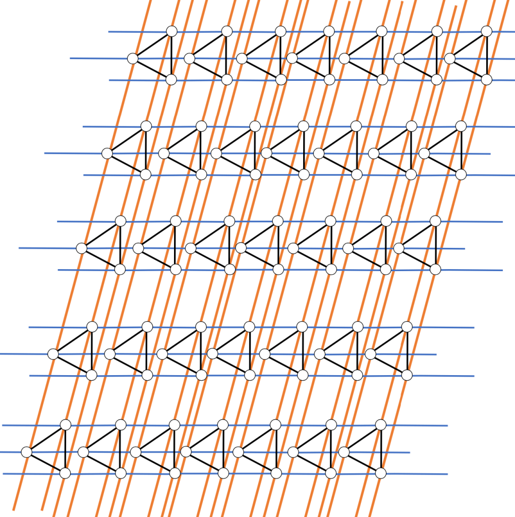
Note the three dotted edges. Each Hamilton double-ray must pass through this edge-set an odd number of times, as otherwise it would have both its ends on the same side of the graph, which in turn would mean it only visits a finite number of vertices on the other side. As this graph is 4-regular, it would be decomposed into two Hamilton double-rays. Two odds add to an even, but there are 3 edges, so clearly this is not possible. This argument can be generalised and refined in the case where our two-ended graph is of the form , namely, a Hamilton decomposition is only possible if is even. What a relief it is then, that it is always possible if is even. The below image suggests the pattern we can apply in such a case.
The Hamilton decomposition of .
The big questions
Erde, Lehner and Pitz 2020 [4]: If and are infinite, finite-degree graphs, each with a Hamilton decomposition into double-rays, then has a Hamilton decomposition into double-rays.
.
In general, it would be nice if has a Hamilton decomposition, this would be a nice generalisation of Foregger’s and Aubert and Schneider’s results for finite graphs, either viewing as an infinite cycle in which case Foregger’s result would apply, or by viewing as the lattice which already has a Hamilton decomposition, in which case Aubert and Schneider’s result would apply. If is even, then we already know that has a Hamilton decomposition as above, so we can use Erde, Lehner and Pitz’s result to then say that has a Hamilton decomposition. If is odd, then doesn’t have a Hamilton decomposition, so we can’t approach it this way. We already know it’s possible for one odd case, namely , in which case we simply have the lattice. Understanding any symmetry and pattern in the even case would be incredibly insightful for determining the odd case, but the construction becomes a bit too complex, and the pictures a bit too messy, that it would take a very careful hand to draw out the decomposition in a way we could wrap our heads around it. If you can manage to draw out the decomposition for , this would already be a more concrete example than anything I have managed to draw, and probably provide quite a valuable mental image of how to translate this to odd . Alternatively, it seems that the simplest odd case has all the right components for its own lovely symmetric solution, given that a decomposition would have 3 colours and the graph has an order 3 symmetry. Such a solution would provide its own insight into the other odd cases. So there is no reason a clever human brain couldn’t figure out a nice solution directly, perhaps inspired by the lattice decomposition. Alas, so far it seems that clever human brain might not be mine, but it might be yours!
Bibliography
[1] Marsha F. Foregger. Hamiltonian decompositions of products of cycles. Discrete Mathematics, 24:251–260, 1978. [2] Jacques Aubert and Bernadette Schneider. Decomposition de la somme cartesienne d’un cycle et de l’union de deux cycles hamiltoniens en cycles hamiltoniens. Discrete Mathematics, 38:7–16, 1982. [3] Richard Stong. Hamilton decompositions of Cartesian products of graphs. Discrete Mathematics, 90:169–190, 1991. [4] Joshua Erde, Florian Lehner, and Max Pitz. Hamilton decompositions of one-ended Cayley graphs. Journal of Combinatorial Theory, B(140):171–191, 2020.


 , the complete graph on 5 vertices. The edges have been coloured so that the edges of one colour form a spanning, 2-regular subgraph. Each colour is called a Hamilton cycle, and the colouring of the graph is called a Hamilton decomposition. A Hamilton cycle provides a path which visits every vertex exactly once and returns to the starting vertex.
  -regular graph must be
  edges which, upon deletion, make the graph disconnected.
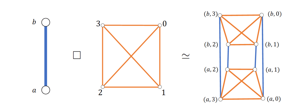
 of two graphs
  and
and  . (
. ( . Check that if
  -regular and
  -regular, then
  -regular.
  .
. 
 has a Hamilton decomposition.
  has a Hamilton decomposition.
 has a Hamilton decomposition.
  the graph which every Hamilton double-ray is isomorphic to.
 -distance graph, which has the integers as vertices, and an edge between two vertices
  iff
iff  .
. 

 -star graph and extending each leaf indefinitely produces a
  :
: 
 , namely, a Hamilton decomposition is only possible if
  is even. What a relief it is then, that it is always possible if
 .
. 
 .
.  has a Hamilton decomposition, this would be a nice generalisation of Foregger’s and Aubert and Schneider’s results for finite graphs, either viewing
  as the lattice which already has a Hamilton decomposition, in which case Aubert and Schneider’s result would apply. If
  , in which case we simply have the lattice. Understanding any symmetry and pattern in the even case would be incredibly insightful for determining the odd case, but the construction becomes a bit too complex, and the pictures a bit too messy, that it would take a very careful hand to draw out the decomposition in a way we could wrap our heads around it. If you can manage to draw out the decomposition for
  , this would already be a more concrete example than anything I have managed to draw, and probably provide quite a valuable mental image of how to translate this to odd
  has all the right components for its own lovely symmetric solution, given that a decomposition would have 3 colours and the graph has an order 3 symmetry. Such a solution would provide its own insight into the other odd cases. So there is no reason a clever human brain couldn’t figure out a nice solution directly, perhaps inspired by the lattice decomposition. Alas, so far it seems that clever human brain might not be mine, but it might be yours!
You must be logged in to post a comment.