dice – Jack Neubecker

See mathsfeed.blog/problem-adding-dice-rolls/ for the motivation, introduction and immediate discussion of the problem.

The problem

We want to roll $N$ dice at a time, and add up the total over repeated rolls, and continue to do so until we reach a threshold $t$ . When we reach or exceed $t$ , we note $X$ , the sum of the dice we just rolled. What is the distribution of $X$ ? We will call the range $t - 6N$ to $t-1$ the striking range, as a roll in this range might get us to $t$ . Inside this range we need to pay extra attention to the value of our dice roll, as depending on its value we might have to roll again, or we might have to stop.

Let $C_{k,N}$ be the cumulative sum of $N$ dice rolled $k$ times. Let $C$ be the cumulative sum of $N$ dice rolled an unknown number of times. We want to find a mixing point $M$ after which $f(c;b) := \mathbb{P} (C = c \mid b \leq C \leq b + 5 N)$ is uniform in terms of $c$ . Why? If we find such an $M$ , then as long as our threshold is at least a few maximum dice rolls away from $M$ , it doesn’t really matter how far away it is, we can always assume our cumulative total approaches the striking range from somewhere uniformly in an appropriately wide interval just outside the striking range. This significantly reduces the complexity of an analytic solution or a computer simulation. If the threshold is not significantly past the mixing point, then we have to be careful as our cumulative total is more likely to be at particular points, and the calculations become more complex, as our cumulative total will come in chunks of about $3.5N$ at a time.

Does M exist?

It might be that $M$ doesn’t really exist, and there is always some very subtle nonuniformity to $f(c;b)$ . This isn’t necessarily the case, but showing that would be another problem entirely, and we’re probably quite fine with $M$ technically a function of some tolerance level. Let’s quickly develop a mental picture with some histograms. This will hopefully convince us that $M$ exists (or we get close enough to uniform that it looks like $M$ exists), and how we might capture its meaning.

Pictures

For a particular set of $k$ and $N$ , $C_{k,N}$ just follows some discrete distribution with a nice bell-curvy shape. Of real interest is sampling from $C$ , as we don’t know how many rolls it took to reach our threshold. The immediate problem is this requires sampling a $k$ first, and we don’t want to have any assumption on $k$ ‘s value. So instead I will just uniformly sample $k$ values between 0 and 200 and hope that our brains can imagine the extension to unbounded $k$ . Play around with my code in the Colab notebook here. Actually, let’s always sample $C_{200,N}$ but keep track of the partial sum at each intermediate step. I know this technically violates independence assumptions, but whatever. I’m also going to work with $N = 20$ for these pictures, as the results are suitably interesting.

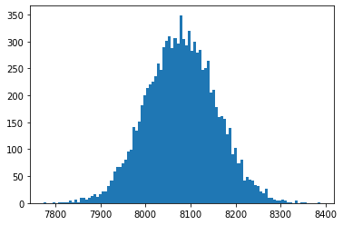
Here we can see a histogram for 10 000 samples of $C_{100, 20}$ . As expected it forms a lovely bell-curve shape.

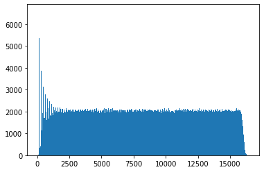
Here we see a histogram for 10 000 samples of $C_{k,20}$ for all $1 \leq k \leq 200$ . We can see the nice uniform property we’re looking for emerge definitively once $C$ exceeds about 3 000, but it’s hard to tell at this scale. Let’s zoom in on the more interesting part of the graph.

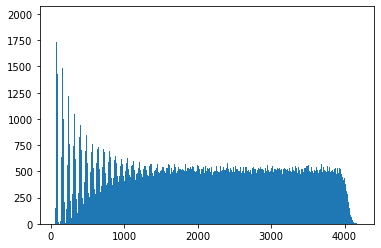
Here we only look at samples of $C_{k,20}$ for $k \leq 50$ . We can see more clearly now the spikes which indicate we are not at the mixing point yet, which we can make out more clearly here is at about $M = 2000$ . Zooming in further:

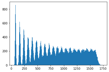
We can identify the spikes more clearly here. Given we roll 20 dice at a time, we should not be surprised to see the initial values occur in spikes about 70 units apart, which is roughly what we see.

They do get a bit wider as we move to the right, as the tails of slightly fatter and further right spikes gently nudge up their neighbours. So, whatever more technical answer we derive below should line up roughly with these observations, namely that by the time $C$ is about 2000, or about 29 dice rolls, it should be well mixed.

Defining M

For a more technical definition, you can be as picky as you like as to how you define suitably uniform, probably with some sort of $\varepsilon$ floating around, but I want a rough and ready answer, and I don’t personally enjoy having $\varepsilon$ ‘s littered throughout my work, so my working definition is as follows:

If, for all $C \geq M$ , it is no longer obvious to infer from $C$ how many rolls $k$ it took to reach $C$ , then $M$ is a mixing point.

Of course this is entirely heuristic, it is not longer obvious (in some sense) as long as there is more than one value $k$ for which $\mathbb{P}(k \mid C)$ is nonzero. This happens very quickly and does not capture what we see in the simulations. In the other direction, for any $C$ , there will always be some much more sensible guesses for $k$ than others, probably an integer close to $\frac{C}{3.5N}$ . So we need to start by deciding on our criteria for obvious. I’ve come up with a couple of different definitions, and I’ll discuss them both below.

Finding M the easier way

It can be checked that $\mathbb{E} C_{k,N} = 3.5 k N$ , and that $var(C_{k,N}) = \frac{35}{12}kN$ . From now on, if I need to, I will approximate $C_{k,N}$ with $\hat{C}_{k,N}$ , a normal random variable with the same mean and variance. Then I can say we have reached the mixing point if there is significant overlap between $C_{k,N}$ and $C_{k+\delta, N}$ for some $\delta \geq 1$ . Again there are lots of choices for what is meant by significant overlap and choice of $\delta$ . Inspired by mathsfeed.blog/is-human-height-bimodal I think a reasonable choice is to compare $\delta = 1$ , and consider the overlap significant if the there is only one mode, not two. Using the fact that a normal pdf is concave down within 1 standard deviation of its mean, we would like that one standard deviation above the mean for $\hat{C}_{k,N}$ :

$3.5 k N + \sqrt{\frac{35}{12} k N}$

is equal to one standard deviation below the mean for $\hat{C}_{k+1,N}$ :

$3.5(k+1)N-\sqrt{\frac{35}{12}(k+1)N}$

One can do some rather boring algebra to arrive at $\sqrt{4.2N} = \sqrt{k+1}+\sqrt{k}$ . You can solve this properly I guess, but I am a deeply lazy person, so I’m going to approximate the right-hand side as $2\sqrt{k}$ . If this upsets you, then I am deeply sorry, but I will not change. ( $k$ is big enough and we’re rounding to a whole number at the end of the day so its fine, but I’ve already spent more time justifying this than I wanted to.) This allows us to arrive at $k \approx 1.05N$ . This roughly agrees with the scale we wanted for $N = 20$ . If you try and count out the first 21 spikes in the above plots, they become very hard to make out by the end. So I’m actually fairly happy with this answer, subject to some proper checking with more choices for $N$ and maybe just topping off with another 20% just for good measure. More important I think is convincing yourself that if I had chosen some other number of standard deviations or some larger $\delta$ , then $k$ as a function of $N$ should still be linear! So instead of rederiving all of these calculations, just remember that if you’re happy $N = 1$ , $t = 500$ is well-mixed, then $N = 10$ , $t = 5000$ should be well-mixed too. Note that this condition truly isn’t enough to guarantee uniformity as it makes no attempt to consider the contribution of any $C_{i,N}$ other than $i = k$ and $i = k + \delta$ , but it should ensure any spikiness is rather muted. If you’re happy with this condition, good, so am I, but I may as well mention the other method I thought of for measuring mixing.

Finding M the bayesian way

The definition of suitably uniform above is very heavily based in conditional probability, and I am a dyed-in-the-wool bayesian, so I’m going to attack with all the bayesian magic spells I can muster. If you’re a committed frequentist, maybe it’s time to look away.

We want to derive

$p(k \mid C) = \frac{p(C,k)}{p(C)}$ .

Can we derive $p(C,k)$ ? Well by the definition of conditional probability,

$p(C,k) = p(k) \cdot p(C \mid k)$ .

I know $p(C \mid k)$ is approximately normal, so

$p(C = c \mid k) \approx \frac{1}{\sqrt{kN\frac{35}{12}2\pi}} \exp{\left(\frac{-1}{2} \frac{1}{kN\frac{35}{12}} (c-3.5kN)^2\right)}$
$\propto \frac{1}{\sqrt{k}} \exp \left( \frac{-1}{k} (c - 3.5kN)^2 \right)$ ,

and we have no prior information about what $k$ should be, so we can treat $p(k)$ with a constant uninformative prior. Finally, $p(C)$ is not a function of $k$ , its just a scaling factor, so

$p(k \mid C) \propto p(C,k) \propto \frac{1}{\sqrt{k}} \exp \left( \frac{-1}{k} (c - 3.5kN)^2 \right)$ .

Now admittedly it’s been a while since I was properly in the stats game, so my tools might be a bit rusty, but this doesn’t look like a pmf I’m familiar with. It looks like it’s in the exponential family, so maybe somebody with more experience in the dark arts can take it from here. I guess you could always figure out some sort of acceptance-rejection sampler if needed. Okay but what’s the point? Well now we have our posterior for $k \mid C$ , we can be more precise about it being suitably non-obvious what to infer for $k$ . The first criteria that come to mind for me is either specifying the variance should be suitably large (which can be approximated up to proportionality with the pdf, though that proportionality depends on $C$ generally), or that the mode of the distribution is suitably unlikely (also easy up to proportionality, but knowing the actual probability itself feels more integral to the interpretation). Of course in both cases we can approximation the proportionality constant by computing an appropriate partial sum. I’ve knocked up a quick demo on Desmos of what this would look like in practice.

Concluding remarks

Note of course that the normal approximation itself only works if the number of dice in each roll is suitably large to apply CLT. It also then feels like no coincidence that ‘about 30 rolls’ is the conclusion, as it sounds an awful lot like my usual usual retort when asked if a sample mean is big enough to make a normal approximation. Overall I’m okay with making approximations which assume a large $N$ for the same reason we are more interested in deriving results for large $t$ , namely for small $t$ and/or $N$ , we can probably simulate the answer with high precision using a computer, or even by hand for very small values. But these asymptotic results help us to be confident in when we can truncate the simulation for speed, or when we can stop doing simulations and rely only on the asymptotic results.

If you enjoyed this, you might enjoy my other posts on problems I would like to see solved, or find out more about my research from my homepage.

Tag: dice

On the problem of adding dice rolls to a threshold