statistics – Jack Neubecker

Why do measure theory in probability?

November 27, 2023November 29, 2023Posted in Blog posts, Probability and Statistics, ResearchTagged expected value, mathematics, measure theory, probability, statistics

What follows is the academic residue of a spirited discussion between a fellow PhD student and myself, concerning the use of measure theory in probability. The central question is “Why bother?” Here is my attempt at an answer to this question, through a small demonstration of measure theory’s ability to generalise. This is not an attempt to teach any measure theory, but I will point to a few resources at the end that I found helpful for reacquainting myself during our discussion if you would like to do the same.

The traditional result

First, we must establish in traditional terms the result we will later emulate measure-theoretically. I will only talk about non-negative random variables; the result generalises by splitting into positive and negative parts, but the notation is drastically simplified.

Theorem 1: If $X$ is a non-negative random variable with density $f(x)$ and probability function $F(x)$ , then $\mathbb{E}(X) = \int_0^{\infty} 1-F(x) dx$ .

Proof:

$\begin{aligned} \int_0^{\infty} 1 - F(x) \mathop{dx} &= \int_0^{\infty} P(X \geq x) \mathop{dx} \\ &= \int_{x=0}^{x=\infty} \int_{u=x}^{u=\infty} f(u) \mathop{du} \mathop{dx} \\ &= \int_{u=0}^{u=\infty} \int_{x=0}^{x=u} f(u) \mathop{dx} \mathop{du} \\ &= \int_{u=0}^{u=\infty} f(u) \int_{x=0}^{x=u} \mathop{dx} \mathop{du} \\ &= \int_{u=0}^{u=\infty} f(u) u \mathop{du} \\ &= \mathbb{E}(X) \end{aligned}$

There are two conceptually important points here. The less theoretically troublesome one is the switching of integrals, which Fubini lets us do, but I’ve always found a little cheeky. More foundationally important is that we assume the existence of a density $f(x)$ here, but it is absent from the result of the theorem. It is an achievable exercise to prove the equivalent result for discrete distributions, and I concede that most continuous distributions I have encountered in the wild have a density, but this does have practical importance. The usefulness of the theorem is in being able to compute an expectation when we don’t have or don’t want to find a density, so it’s essentially useless if having a density is a pre-condition to its application. Can we get around this somehow?

In steps measure theory

I will spare the majority of the details of satisfactorily defining a random variable measure-theoretically, but some objects need to be defined.

The premise of measure-theoretic probability is that we start with a measure space $\left(\Omega, E, \mathbb{P} \right)$ . In probability terms, this gives us a sample space $\Omega$ , a set of events $E$ and a probability measure $\mathbb{P}$ , as long as $\int_{\Omega} d \mathbb{P} = 1$ . We will brush over what $\int_{\Omega} d \mathbb{P} = 1$ is really saying, but suffice to say it imposes Kolmogorov’s unit measure axiom. The other axioms of probability are packaged up in what a measure space is. This gives us a notion of what probability means on $\Omega$ . We can then define a real-valued random variable as a measurable function from $\Omega$ to the reals, that is, a function $f: \Omega \to \mathbb{R}$ such that the pre-image $f^{-1}((a,b))$ of any open interval $(a,b)$ is an element of $E$ .

For our purposes, we can define any real-valued random variable as follows, by first defining the $\mathrm{Uniform}\left(0,1\right)$ distribution. Take $\left(\left[0,1\right], \lambda\left(\left[0,1\right]\right), \mu \right)$ to be our measure space, where $\lambda\left(\left[0,1]\right]\right)$ is the set of Lebesgue-measurable subsets of $\left[0,1\right]$ , and $\mu$ is the Lebesgue measure. Then the uniform distribution $U$ can be defined as the identity map $U: \left[0,1\right] \to \left[0,1\right] ; U(\omega) = \omega$ . You can check for yourself that any property you like about the uniform distribution carries over perfectly. In particular, we can check that $P\left(a \leq U \leq b\right) = \mu\left( \left( a,b \right) \right) = b-a$ .

Now, anyone familiar with the inverse-transform will know that defining any other real-valued random variable is a piece of cake. Every real-valued random variable $X$ has a distribution function $P\left(X \leq x\right) = F_X(x)$ , so we define $X : \left[0,1\right] \to \mathbb{R}; X(\omega) =F_X^{-1} \circ U(\omega) = F_X^{-1}(\omega)$ . $F_X^{-1}$ might not be easy to compute, but it definitely exists.

We are still missing one key element, expected value. We define it as $\mathbb{E}(X) = \int_\Omega X d \mathbb{P}$ . I will leave undefined what it means to actually compute an integral this way, but it can be done. Importantly, it is still achieving the same goal of finding area under a curve. We are now ready to prove:

Theorem 2: If $X$ is a non-negative random variable with probability function $F(x)$ , then $\mathbb{E}(X) = \int_0^{\infty} 1-F(x) dx$ .

Proof:

If you’ll allow me a couple of pictures, I argue that it is true by definition. We see that the area integrated by $\int_0^{\infty} 1 - F(x) dx$ and the area integrated by $\int_{\left[0,1\right]} F^{-1} \mathop{d\mu}$ are in fact the same areas.

$\int_{\left[0,1\right]} F^{-1} \mathop{d\mu}$ .

Q.E.D.

Some healthy skepticism

Now, we should be skeptical of any proof which follows so readily from the definitions. The traditional discrete distribution is marvelously intuitive. Further, we can squint at the traditional continuous expected value definition and notice the pattern. By comparison, the measure-theoretic definition is quite opaque. So far it seems like we just made up a definition so that this proof was easy. What’s the value in that? Here’s how I see it.

I liken it to the intermediate value theorem (IVT). The point of proving the IVT is not to dispel any doubt that if an arrow pierces my heart it must also have pierced my ribcage. The point of the IVT is in showing that the definition of mathematical continuity we have written down captures the same notion of physical and temporal continuity we sense in the real world.

What we have really learned from theorem 2 then, is that we can define expected value in terms of the probability function directly. We essentially drop the density assumption by fiat. The value is in discovering this more powerful definition which unites previously disparate discrete and continuous cases, as well as distributions which are a mix of both.

A concrete mixed distribution example

My favourite mixed distribution is the zero-inflated exponential, with probability function $F(x) = p + (1-p)(1-e^{-\lambda x})$ when $x \geq 0$ , and $0$ otherwise.

Traditionally, to evaluate an expected value we would have to be rather careful or apply some clever insight. Now with measure theory, we can ham-fistedly shove $F(x)$ straight in to $\int_0^{\infty} 1-F(x) \mathop{dx}$ and call it a day.

We can also start sparring with more exotic random variables on non-numeric spaces with confidence. I’m currently working through Diaconis’ Group Representations in Probability and Statistics, so hopefully I can speak on these “applications” in more detail in the future. But for now, I’ll leave it as an enticing mountaintop rather than trying to spoil the ending.

Intuition

It is no secret that I don’t like the IVT, or theorem-motivated definitions more broadly, so I am uncomfortable leaning on it in an argument. What I will provide here is my own post-hoc intuition for the measure-theoretic expected value. Rather fortuitously it leans on the IVT, so I’ll point out pedantically that I’m actually using it as the Intermediate Value Property (IVP) in and of itself. Observe below that the area on the left is the area defining a measure-theoretic expected value as we have seen above.

The area defining a measure-theoretic expected value, and the rectangular region of equal area guaranteed by the IVP.

Note that this area is the same as the area of the rectangular region. As it has unit width, its height is also its area. This height is not coincidentally the mean value of $F_X^{-1}$ guaranteed by the IVP, so we see that the measure-theoretic definition gives us a measure of central tendency. That this is the same measure of central tendency as the traditional definition can be shown in many ways, but we have seen it today as a porism of theorem 2.

What have we learned?

In short, that generalisation is cool, and measure theory is not as scary as I thought after failing it in third-year. It gives us steady footing to go and explore exotic spaces, and it provides some nice perspectives on old favourites. Is it of practical use to the working statistician? Debateable. Our main theorem can certainly be used without actually doing any measure. Perhaps it provides nice perspectives on transformations if one does need to compute certain integrals which aren’t recognisable. What do you think? Have I convinced you measure-theoretic probability isn’t useless? Do you know any interesting applications I didn’t mention? As always, I’d love to hear your thoughts.

Resources

I am always hesitant to endorse texts based solely on how helpful they were to me. We should remember that one always understands something better the second time. That being said, the following two probability-oriented texts were useful to me. Matthew N. Bernstein has a trio of nice blog posts entitled Demystifying measure-theoretic probability theory, which are a nice, slow introduction to some of the basics. I also found Sebastien Roch’s Lecture Notes on Measure-theoretic Probability Theory useful as a much denser, more comprehensive reference. As for strictly measure-theoretic principles, I found plenty enough information by simply clicking the first Wikipedia article to pop up when I searched the relevant terms.

On the problem of adding dice rolls to a threshold

May 9, 2022November 29, 2023Posted in Blog posts, Probability and Statistics, Problems I would like to see solvedTagged bayesian inference, chance, dice, mathematics, probability, problem solving, recreational mathematics, simulation, statistics

See mathsfeed.blog/problem-adding-dice-rolls/ for the motivation, introduction and immediate discussion of the problem.

The problem

We want to roll $N$ dice at a time, and add up the total over repeated rolls, and continue to do so until we reach a threshold $t$ . When we reach or exceed $t$ , we note $X$ , the sum of the dice we just rolled. What is the distribution of $X$ ? We will call the range $t - 6N$ to $t-1$ the striking range, as a roll in this range might get us to $t$ . Inside this range we need to pay extra attention to the value of our dice roll, as depending on its value we might have to roll again, or we might have to stop.

Let $C_{k,N}$ be the cumulative sum of $N$ dice rolled $k$ times. Let $C$ be the cumulative sum of $N$ dice rolled an unknown number of times. We want to find a mixing point $M$ after which $f(c;b) := \mathbb{P} (C = c \mid b \leq C \leq b + 5 N)$ is uniform in terms of $c$ . Why? If we find such an $M$ , then as long as our threshold is at least a few maximum dice rolls away from $M$ , it doesn’t really matter how far away it is, we can always assume our cumulative total approaches the striking range from somewhere uniformly in an appropriately wide interval just outside the striking range. This significantly reduces the complexity of an analytic solution or a computer simulation. If the threshold is not significantly past the mixing point, then we have to be careful as our cumulative total is more likely to be at particular points, and the calculations become more complex, as our cumulative total will come in chunks of about $3.5N$ at a time.

Does M exist?

It might be that $M$ doesn’t really exist, and there is always some very subtle nonuniformity to $f(c;b)$ . This isn’t necessarily the case, but showing that would be another problem entirely, and we’re probably quite fine with $M$ technically a function of some tolerance level. Let’s quickly develop a mental picture with some histograms. This will hopefully convince us that $M$ exists (or we get close enough to uniform that it looks like $M$ exists), and how we might capture its meaning.

Pictures

For a particular set of $k$ and $N$ , $C_{k,N}$ just follows some discrete distribution with a nice bell-curvy shape. Of real interest is sampling from $C$ , as we don’t know how many rolls it took to reach our threshold. The immediate problem is this requires sampling a $k$ first, and we don’t want to have any assumption on $k$ ‘s value. So instead I will just uniformly sample $k$ values between 0 and 200 and hope that our brains can imagine the extension to unbounded $k$ . Play around with my code in the Colab notebook here. Actually, let’s always sample $C_{200,N}$ but keep track of the partial sum at each intermediate step. I know this technically violates independence assumptions, but whatever. I’m also going to work with $N = 20$ for these pictures, as the results are suitably interesting.

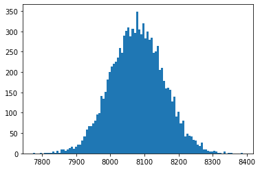
Here we can see a histogram for 10 000 samples of $C_{100, 20}$ . As expected it forms a lovely bell-curve shape.

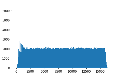
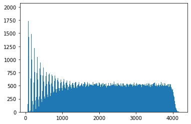
Here we see a histogram for 10 000 samples of $C_{k,20}$ for all $1 \leq k \leq 200$ . We can see the nice uniform property we’re looking for emerge definitively once $C$ exceeds about 3 000, but it’s hard to tell at this scale. Let’s zoom in on the more interesting part of the graph.

Here we only look at samples of $C_{k,20}$ for $k \leq 50$ . We can see more clearly now the spikes which indicate we are not at the mixing point yet, which we can make out more clearly here is at about $M = 2000$ . Zooming in further:

We can identify the spikes more clearly here. Given we roll 20 dice at a time, we should not be surprised to see the initial values occur in spikes about 70 units apart, which is roughly what we see.

They do get a bit wider as we move to the right, as the tails of slightly fatter and further right spikes gently nudge up their neighbours. So, whatever more technical answer we derive below should line up roughly with these observations, namely that by the time $C$ is about 2000, or about 29 dice rolls, it should be well mixed.

Defining M

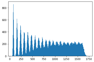
For a more technical definition, you can be as picky as you like as to how you define suitably uniform, probably with some sort of $\varepsilon$ floating around, but I want a rough and ready answer, and I don’t personally enjoy having $\varepsilon$ ‘s littered throughout my work, so my working definition is as follows:

If, for all $C \geq M$ , it is no longer obvious to infer from $C$ how many rolls $k$ it took to reach $C$ , then $M$ is a mixing point.

Of course this is entirely heuristic, it is not longer obvious (in some sense) as long as there is more than one value $k$ for which $\mathbb{P}(k \mid C)$ is nonzero. This happens very quickly and does not capture what we see in the simulations. In the other direction, for any $C$ , there will always be some much more sensible guesses for $k$ than others, probably an integer close to $\frac{C}{3.5N}$ . So we need to start by deciding on our criteria for obvious. I’ve come up with a couple of different definitions, and I’ll discuss them both below.

Finding M the easier way

It can be checked that $\mathbb{E} C_{k,N} = 3.5 k N$ , and that $var(C_{k,N}) = \frac{35}{12}kN$ . From now on, if I need to, I will approximate $C_{k,N}$ with $\hat{C}_{k,N}$ , a normal random variable with the same mean and variance. Then I can say we have reached the mixing point if there is significant overlap between $C_{k,N}$ and $C_{k+\delta, N}$ for some $\delta \geq 1$ . Again there are lots of choices for what is meant by significant overlap and choice of $\delta$ . Inspired by mathsfeed.blog/is-human-height-bimodal I think a reasonable choice is to compare $\delta = 1$ , and consider the overlap significant if the there is only one mode, not two. Using the fact that a normal pdf is concave down within 1 standard deviation of its mean, we would like that one standard deviation above the mean for $\hat{C}_{k,N}$ :

$3.5 k N + \sqrt{\frac{35}{12} k N}$

is equal to one standard deviation below the mean for $\hat{C}_{k+1,N}$ :

$3.5(k+1)N-\sqrt{\frac{35}{12}(k+1)N}$

One can do some rather boring algebra to arrive at $\sqrt{4.2N} = \sqrt{k+1}+\sqrt{k}$ . You can solve this properly I guess, but I am a deeply lazy person, so I’m going to approximate the right-hand side as $2\sqrt{k}$ . If this upsets you, then I am deeply sorry, but I will not change. ( $k$ is big enough and we’re rounding to a whole number at the end of the day so its fine, but I’ve already spent more time justifying this than I wanted to.) This allows us to arrive at $k \approx 1.05N$ . This roughly agrees with the scale we wanted for $N = 20$ . If you try and count out the first 21 spikes in the above plots, they become very hard to make out by the end. So I’m actually fairly happy with this answer, subject to some proper checking with more choices for $N$ and maybe just topping off with another 20% just for good measure. More important I think is convincing yourself that if I had chosen some other number of standard deviations or some larger $\delta$ , then $k$ as a function of $N$ should still be linear! So instead of rederiving all of these calculations, just remember that if you’re happy $N = 1$ , $t = 500$ is well-mixed, then $N = 10$ , $t = 5000$ should be well-mixed too. Note that this condition truly isn’t enough to guarantee uniformity as it makes no attempt to consider the contribution of any $C_{i,N}$ other than $i = k$ and $i = k + \delta$ , but it should ensure any spikiness is rather muted. If you’re happy with this condition, good, so am I, but I may as well mention the other method I thought of for measuring mixing.

Finding M the bayesian way

The definition of suitably uniform above is very heavily based in conditional probability, and I am a dyed-in-the-wool bayesian, so I’m going to attack with all the bayesian magic spells I can muster. If you’re a committed frequentist, maybe it’s time to look away.

We want to derive

$p(k \mid C) = \frac{p(C,k)}{p(C)}$ .

Can we derive $p(C,k)$ ? Well by the definition of conditional probability,

$p(C,k) = p(k) \cdot p(C \mid k)$ .

I know $p(C \mid k)$ is approximately normal, so

$p(C = c \mid k) \approx \frac{1}{\sqrt{kN\frac{35}{12}2\pi}} \exp{\left(\frac{-1}{2} \frac{1}{kN\frac{35}{12}} (c-3.5kN)^2\right)}$
$\propto \frac{1}{\sqrt{k}} \exp \left( \frac{-1}{k} (c - 3.5kN)^2 \right)$ ,

and we have no prior information about what $k$ should be, so we can treat $p(k)$ with a constant uninformative prior. Finally, $p(C)$ is not a function of $k$ , its just a scaling factor, so

$p(k \mid C) \propto p(C,k) \propto \frac{1}{\sqrt{k}} \exp \left( \frac{-1}{k} (c - 3.5kN)^2 \right)$ .

Now admittedly it’s been a while since I was properly in the stats game, so my tools might be a bit rusty, but this doesn’t look like a pmf I’m familiar with. It looks like it’s in the exponential family, so maybe somebody with more experience in the dark arts can take it from here. I guess you could always figure out some sort of acceptance-rejection sampler if needed. Okay but what’s the point? Well now we have our posterior for $k \mid C$ , we can be more precise about it being suitably non-obvious what to infer for $k$ . The first criteria that come to mind for me is either specifying the variance should be suitably large (which can be approximated up to proportionality with the pdf, though that proportionality depends on $C$ generally), or that the mode of the distribution is suitably unlikely (also easy up to proportionality, but knowing the actual probability itself feels more integral to the interpretation). Of course in both cases we can approximation the proportionality constant by computing an appropriate partial sum. I’ve knocked up a quick demo on Desmos of what this would look like in practice.

Concluding remarks

Note of course that the normal approximation itself only works if the number of dice in each roll is suitably large to apply CLT. It also then feels like no coincidence that ‘about 30 rolls’ is the conclusion, as it sounds an awful lot like my usual usual retort when asked if a sample mean is big enough to make a normal approximation. Overall I’m okay with making approximations which assume a large $N$ for the same reason we are more interested in deriving results for large $t$ , namely for small $t$ and/or $N$ , we can probably simulate the answer with high precision using a computer, or even by hand for very small values. But these asymptotic results help us to be confident in when we can truncate the simulation for speed, or when we can stop doing simulations and rely only on the asymptotic results.

If you enjoyed this, you might enjoy my other posts on problems I would like to see solved, or find out more about my research from my homepage.